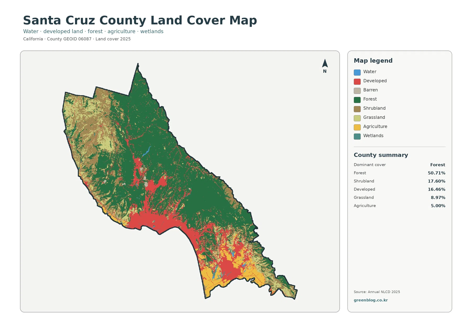
The Santa Cruz County California Land Cover Map is dominated by forest rather than urban cover. Forest accounts for 50.71% of the 2025 classification, while shrubland covers 17.60%, developed land 16.46%, grassland 8.97%, and agriculture 5.00%. The strongest visual contrast is between the wooded Santa Cruz Mountains and the more developed and farmed areas closer to the coast and Pajaro Valley.
Four matching views are provided here: the full 2025 land-cover classification, a forest-and-farmland emphasis map, fractional impervious surface, and a 1985–2025 class-comparison map. The article uses 1800 × 1273 WebP previews, and the four original 2480 × 1754 JPG maps are available in one download. They are useful for comparing countywide patterns, but they are not parcel maps, zoning records, or survey data.
Table of Contents
A forested county between mountain slopes and a busy coast
A first look at the 2025 classification puts Santa Cruz County in a different light from the image of a compact coastal urban area. More than half of the mapped county is forest. Much of that green cover occupies the northern and eastern mountain terrain, while the developed class becomes more prominent toward the central coast and the southeastern end of the county. Shrub and grass cover fill many of the more open upland and coastal areas between those larger blocks.
| Forest, 2025 | 50.71% |
|---|---|
| Shrubland, 2025 | 17.60% |
| Developed, 2025 | 16.46% |
| Grassland, 2025 | 8.97% |
| Agriculture, 2025 | 5.00% |
| Wetlands, 2025 | 0.66% |
| Water, 2025 | 0.30% |
The central coastal developed area stands out because its red tones are compact and bright, not because it occupies most of the county. A second substantial developed concentration appears around the Watsonville side of the county. Between and behind those urban areas, forest, shrub, and grass classes quickly become more common. The result is a county where developed land is locally dense but still surrounded by a much larger natural-cover matrix.
Santa Cruz County planning documents describe the Santa Cruz Mountains and inter-mountain valleys as supporting extensive forest resources. The county General Plan also notes more than 90,000 acres designated as timber resource lands. That planning designation should not be confused with the 50.71% NLCD forest value: one is a legal or resource-management designation, while the other is a remotely sensed surface-cover classification. The two sources are useful together only when their different purposes are kept clear.
Pajaro Valley agriculture is small in countywide area but highly concentrated
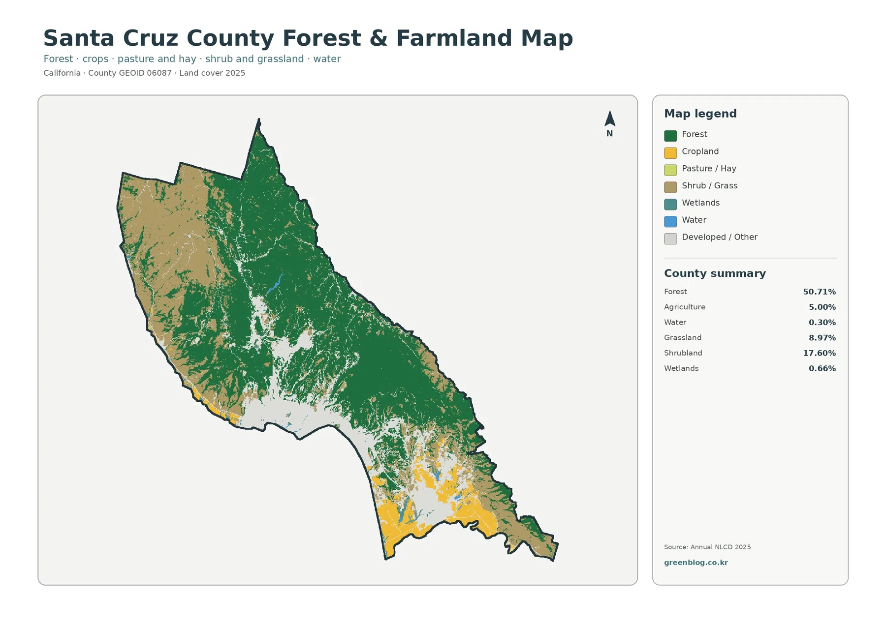
Agriculture makes up 5.00% of the county in the supplied 2025 summary. That number looks modest beside forest and shrubland, yet the forest-and-farmland view makes the agricultural geography easy to locate. Yellow cropland is especially visible in the southeastern lowlands around Watsonville and Pajaro Valley, with additional smaller agricultural areas along parts of the coast. The northern and eastern mountains remain overwhelmingly green in this simplified view.
The location matters because land-cover percentage is not a measure of economic importance. Santa Cruz County’s 2024 Crop Report lists $741.917 million in gross agricultural production value. Berries—strawberries, raspberries, and blackberries—represented 60% of that value, and the report specifically notes blackberry production around Watsonville and Pajaro Valley. The map and crop report therefore describe different dimensions of the same county: one shows surface location, while the other measures agricultural production.
This distinction also prevents a common map-reading mistake. A yellow agricultural cell does not identify a farm parcel, owner, crop contract, conservation easement, or zoning category. Likewise, land mapped as forest is not automatically public land or timber-production property. Annual NLCD classifies what is covering the ground at the observation scale; legal land use and property status come from separate county records.
Wetland and water classes are small in the county summary—0.66% and 0.30%—but narrow waterways and wet areas can still matter locally. Because the product is generalized to raster cells, small streams, drainage channels, and complex wetland edges may not be drawn at field-survey precision. The forest-and-farmland map is best used for broad comparison, then supplemented with dedicated hydrology or wetland data when the question becomes site specific.
Two urban concentrations stand out in the impervious-surface layer
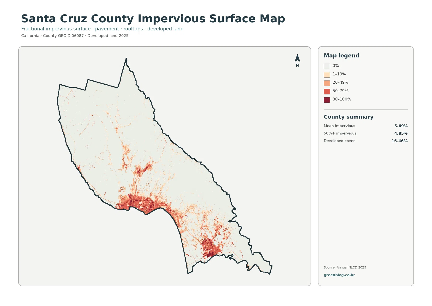
Impervious surface measures hard cover such as pavement, parking areas, and rooftops that does not readily absorb rainfall. The countywide mean is 5.69%, and 4.85% of the mapped area falls in cells with at least 50% impervious surface. These figures are lower than the 16.46% developed-land share because the two products measure different things. A developed cell can still contain trees, lawns, bare soil, and other permeable ground.
The strongest hard-surface concentration follows the central coastal urban area around Santa Cruz and Capitola, with connected developed areas extending through nearby unincorporated communities. Another dense cluster appears around Watsonville in the southeast. Farther into the mountains, red and orange tones become sparse and usually occur as small settlement patches or thin linear features rather than broad urban blocks.
County planning material similarly identifies higher-intensity urban concentrations in the incorporated cities and in unincorporated communities such as Live Oak, Soquel, Seacliff/Aptos, and Rio Del Mar. The impervious layer is consistent with that coastal concentration, but it should not be used to draw municipal limits. It depicts surface hardness, not jurisdictional boundaries, service areas, or legal development entitlements.
For watershed or environmental education, the layer makes a useful contrast with the forest map. Students can compare a highly impervious coastal cell with a mostly forested mountain cell and immediately see that “developed” is not a single uniform surface condition. Engineering conclusions require more information, however. Runoff and flood behavior also depend on slope, soil, drainage infrastructure, rainfall, channels, and other local conditions.
The long-term comparison has a large forest-class signal
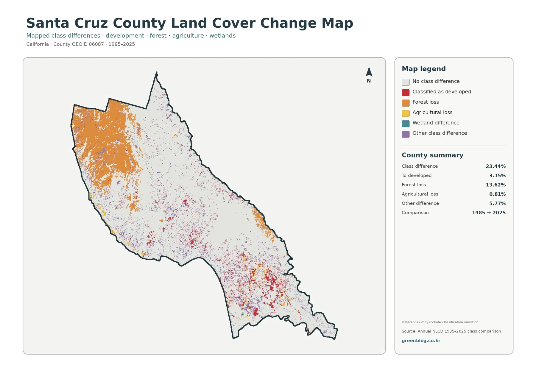
The 1985–2025 comparison marks class differences rather than providing a complete history of land use. The county summary reports class difference across 23.44% of the mapped area. Of that comparison, 3.15% is summarized as change to developed, 13.62% as forest loss, 0.81% as agricultural loss, and 5.77% as other class difference. A wetland-difference category also appears in the legend, but the supplied summary does not give it a separate percentage, so no additional value should be inferred.
Orange forest-change pixels are especially widespread in the northwestern portion of the county and appear in other mountain areas as well. The label “forest loss” is easy to overread. It means a cell that was classified as forest in 1985 is classified as something else in 2025; it does not establish logging, permanent clearing, or ecological degradation as the cause. Fire, vegetation succession, regrowth timing, transitions between forest and shrub classes, and classification differences can all affect a four-decade comparison.
Developed-change pixels are more concentrated near existing urban areas, including the central coast and the Watsonville side of the county. Their location can help identify places worth investigating with historical imagery or planning records, but the map does not say whether housing, commercial construction, road work, or another process produced the class change. Spatial coincidence should not be converted into a causal statement without another source.
Agricultural loss at 0.81% needs the same caution. A changed cell might reflect rotation, fallow conditions, a temporary cover difference, conversion to another class, or classification uncertainty. The most defensible use of the map is to locate change signals first and then ask a more specific question with aerial photographs, fire history, agricultural records, or local planning documents.
Using the four files together without losing location
A reliable comparison starts with the general 2025 map. Locate the broad mountain forest, the central coastal developed area, and the Watsonville–Pajaro Valley agricultural and urban zone. Those three reference areas are visually distinctive enough to carry into the other files. Once the major locations are fixed, smaller shrub, grass, wetland, and water patches are easier to interpret without confusing one part of the county for another.
Switch next to the forest-and-farmland image when the question concerns natural and agricultural cover. It removes some of the detail from the developed categories and makes the contrast between wooded mountains and southeastern farmland clearer. A report about agriculture can pair that map with the county Crop Report, while a forest discussion can pair it with the General Plan’s resource information. Neither combination turns the map into a parcel-level inventory.
The impervious file works best after the developed class has already been located. Compare the 16.46% developed share with the 5.69% mean impervious value and examine where high percentages actually cluster. This sequence explains why a residential area with vegetation can be classified as developed without being 100% pavement and rooftops. It also keeps the focus on observed surface cover rather than assumptions about population or zoning.
Finish with the change map when a historical question is being formed. Instead of treating every colored change pixel as a conclusion, use clusters as prompts for follow-up. Forest-change areas can be checked against fire and vegetation records, while developed-change areas can be compared with archived imagery or planning documents. The four-map workflow is most valuable when each file narrows the next question rather than repeating the same statement.
Why 30-meter cells need careful interpretation
Annual NLCD is a raster dataset commonly produced at 30-meter resolution. Raster data divide the landscape into square cells and assign a class or value to each cell. That scale works well for countywide patterns, but a 30-meter cell is too coarse to reproduce every driveway, narrow creek, field edge, or small patch of vegetation exactly. The clean colored boundary in the graphic is therefore more precise-looking than the underlying landscape may be.
Mixed pixels are unavoidable at many edges. A cell beside a neighborhood may contain a roof, trees, grass, and pavement; a cell near a riparian corridor may contain water and vegetation. Classification must simplify that mixture into a defined land-cover class or an impervious fraction. Small differences along boundaries should not be treated as surveyed changes on the ground.
Date is another limitation. The first three maps represent 2025 conditions in the supplied package, while the historical graphic compares 1985 with 2025. Fire, recovery, construction, crop rotation, restoration, or other events after the observation year are absent. Anyone using the map for a current project should check whether newer local imagery or site information is available.
Property and regulatory questions require a different source entirely. These graphics do not identify assessor parcels, ownership, zoning, building permits, legal access, conservation easements, or surveyed boundaries. Santa Cruz County GIS provides many of those planning layers separately and cautions that mapped information can vary in accuracy. Use the land-cover set for environmental and geographic context, then move to the appropriate official record for a legal or site-specific decision.
Download the four original Santa Cruz County JPG maps
Choose the general land-cover JPG for a full 2025 class overview, the forest-and-farmland file when those two cover types need extra emphasis, and the impervious map when the concentration of pavement and rooftops is the main subject. The change JPG is the historical comparison file and should retain its 1985–2025 label whenever it is reused in a report or presentation.
Each original is 2480 × 1754 pixels. The asset manifest does not mark these images as meeting its A3 high-resolution reference, so test the legend and small text at the intended print size before producing large copies. The download contains JPG images only; it does not include vector artwork, GIS layers, parcel files, or the editable project used to create the maps.
Frequently Asked Questions
Does 50.71% forest mean half the county is legally designated forest land?
No. The percentage describes surface cover classified as forest in the 2025 Annual NLCD product. Timber resource land, parks, private forest, conservation land, and zoning are separate legal or planning categories. Santa Cruz County planning and GIS records are needed for those questions.
Why does agriculture matter if it covers only 5.00% of the map?
The 5.00% figure is an area share, not an economic measure. Agricultural cover is concentrated around Pajaro Valley and Watsonville, and the county’s 2024 Crop Report lists about $741.9 million in gross agricultural production value. A small countywide land-cover percentage can therefore represent a locally concentrated and economically important landscape.
Is the 13.62% forest-loss category proof of deforestation?
No. It records cells that were classified as forest in 1985 and as another class in 2025. The supplied change map warns that differences may include classification variation, and it does not identify a cause. Fire, succession, regrowth timing, class transitions, and real land-cover conversion all require separate evidence.
Map File Information
The ZIP contains one original JPG for each of the four Santa Cruz County land-cover views discussed on this page. Every file is 2480 × 1754 pixels, giving you the original map image rather than the smaller WebP preview used in the article.
- Included Files: 2025 land cover · Forest and farmland · Impervious surface · 1985–2025 land-cover change
- File Type: Four JPG files in one ZIP archive
Related Maps
- Alameda County California Land Cover Map
- Alpine County California Land Cover Map
- Amador County California Land Cover Map
Sources and Reference
These official resources provide the dataset definitions and local forest, planning, and agricultural context used to interpret the supplied maps. They are also useful starting points when a county-scale graphic needs to be supplemented with current or site-specific information.
- MRLC Annual NLCD Data — official access point for Annual NLCD land-cover and related products.
- USGS Annual NLCD Land Cover Classification — official explanation of land-cover classes and classification context.
- County of Santa Cruz General, Town & Village Plans — 2024 General Plan and local planning context for natural resources and urban/rural areas.
- Santa Cruz County Annual Crop and Livestock Reports — official annual crop reports including 2024 production values and commodity information.
- U.S. Census Bureau TIGER/Line Shapefiles — official county boundary and geographic identifier reference.
Green Map creates custom-edited map images using open geographic data sources such as geoBoundaries, Natural Earth, OpenStreetMap, and government open data.
These maps are edited visual materials, not raw data files, and are provided for education, documents, presentations, and graphic reference.