The Calaveras County California Land Cover Map set captures a strong west-to-east contrast. Open shrub and grass cover occupies much of the western side, while forest becomes the dominant surface across the higher eastern part of the county. The 2025 summary lists forest at 39.86%, shrubland at 28.03%, and grassland at 23.80%, with developed land at 5.74% and water at 2.05%.
Four map views are available on this page: current land cover, forest and farmland, impervious surface and developed land, and a 1985–2025 land-cover comparison. The four original JPG maps are also packaged in one download. Together they help separate broad vegetation patterns from built surfaces and make it easier to see where long-term class differences are concentrated.
Table of Contents
A county that changes from open western country to a forested east
Calaveras County does not have one uniform land-cover pattern. The western portion contains broad areas of grassland and shrubland, with developed patches and water features breaking up the open cover. Moving east, forest becomes increasingly common until large connected areas of green occupy most of the eastern extension. The transition is gradual through the middle of the county, where forest, shrubland, and grassland form an irregular mosaic rather than a sharp dividing line.
The county’s own planning documents describe a similar landscape contrast. Calaveras County’s General Plan environmental material notes large open ranching landscapes in the western part of the county and more prevalent forest landscapes in the higher-elevation east. That local description is useful context for the 2025 land-cover map because the mapped classes follow the same broad geographic change without requiring every open area to be interpreted as a single legal or economic land use.
Forest is the largest mapped class at 39.86%, but its importance is even more obvious spatially than the countywide percentage suggests. It forms a broad, mostly connected region across the east and northeast. Shrubland, which accounts for 28.03%, is much more prominent in the west and central transition zone. Grassland at 23.80% fills extensive western areas and appears in smaller openings farther east.
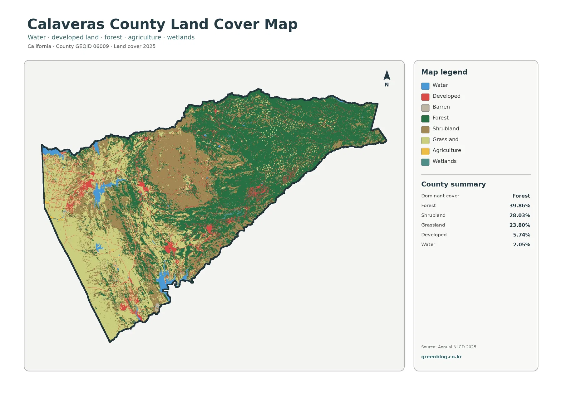
Developed land makes up 5.74% of the county. Instead of forming one large urban block, it appears in several clusters and narrow connections, especially in the western and south-central portions. Those red patches are small compared with the natural cover around them, yet they stand out because most of the county is not classified as developed. Farther into the eastern forest, developed pixels become sparse and more isolated.
Water accounts for 2.05% of the 2025 summary. Several blue water bodies are easy to locate on the western and central portions of the map, and another water feature appears close to the southern boundary. Their shapes make useful orientation points when comparing the four map products. A water body that is surrounded by open cover on one map can be checked against forest, development, and change patterns in the same location on the others.
Built surfaces occupy a small share but form clear local clusters
The impervious-surface map narrows the question from “where is land developed?” to “where are hard surfaces concentrated?” Impervious surfaces include pavement, rooftops, parking areas, and other materials that do not readily absorb water. Calaveras County has a mean impervious value of 1.07% in the supplied 2025 summary, while only 0.29% of the county is shown at 50% impervious or greater.
Those low countywide values do not mean every part of Calaveras County is equally unpaved. Orange and red pixels are concentrated in compact settlement areas and along thin developed connections, while most large forest and open-land areas remain near zero. The contrast is especially strong when the impervious map is viewed immediately after the full land-cover map: developed places that are obvious in red on the first sheet become smaller, more detailed concentrations of hard surface on the second.
The difference between 5.74% developed cover and a 1.07% mean impervious surface is important. A developed land-cover class can include lawns, trees, bare soil, and other permeable ground mixed with buildings and roads. The impervious product measures the hard-surface fraction rather than treating the entire developed cell as pavement. A low-density residential area can therefore be classified as developed even though most of its ground surface still absorbs water.
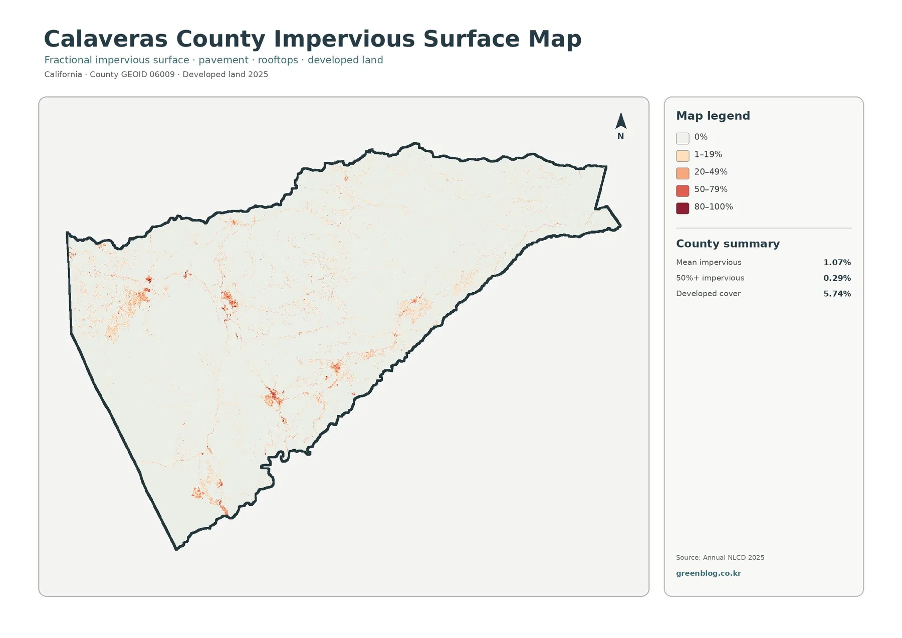
This map is useful for comparing settlement intensity, but it is not a building or parcel inventory. Annual NLCD is a raster product, so a 30-meter cell can contain several real surfaces at once. A road may occupy only part of a cell, and a house may share the same cell with trees or soil. The map is best read at neighborhood-to-county scale rather than as a measurement of an individual lot.
Forest and open cover explain more than the tiny agriculture class
The forest-and-farmland view simplifies the county into a smaller set of classes. Forest remains the largest single category at 39.86%, while grassland and shrubland continue to occupy much of the western half. Agriculture is listed at just 0.11%, wetlands at 0.27%, and water at 2.05%. The simplified colors make the boundary between forested uplands and open western country easier to follow than on the full land-cover sheet.
The 0.11% agriculture figure needs careful interpretation. Land cover is not the same thing as agricultural use, zoning, ownership, or a county’s agricultural economy. Ground used for grazing can still be classified as grassland or shrubland when that is the surface visible to the land-cover model. Calaveras County’s official resource-planning documents discuss ranching and agricultural production as important local activities, so the mapped agriculture class should not be used as a direct estimate of all land participating in agriculture.
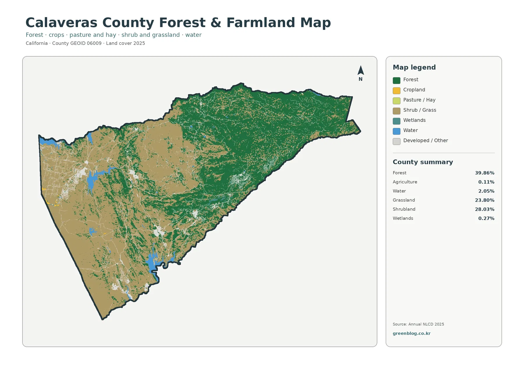
The map also shows why percentages alone can hide local structure. Forest is 39.86% countywide, yet in the eastern portion it visually occupies far more than 39.86% of the immediate landscape. Grassland and shrubland behave the same way in the west, where they dominate large local areas even though their countywide percentages are lower than forest. Reading location and percentage together gives a much better picture than ranking the classes by number.
Wetlands are only 0.27% in the summary, so they appear as small and narrow features rather than a major countywide block. Water is more visible, but it is still a minor class by area. These small categories can matter greatly for watershed or habitat studies, which is why the location of a wetland or water edge can be more useful than its share of the county. At 30-meter resolution, narrow features should still be treated as generalized rather than exact boundaries.
The 1985–2025 comparison is dominated by forest-class differences
The change map compares the class assigned in 1985 with the class assigned in 2025. Its summary reports class differences across 22.83% of Calaveras County. Forest loss is the largest labeled component at 11.11%. Changes classified as “to developed” account for 2.43%, agricultural loss is 0.03%, and other class differences account for 9.23%.
A large orange area is immediately visible in the north-central portion of the county, with smaller forest-difference patches extending elsewhere through the center and east. The current 2025 map still shows substantial forest around and beyond many of these areas. For that reason, the orange class should be read as a difference between two classified dates, not as proof that every pixel represents permanent deforestation.
The map itself warns that the differences may include classification variation. Over a forty-year comparison, a cell may move between forest, shrub, and grass classes because vegetation changed, because recovery or disturbance altered the dominant cover, or because the classification system handled a mixed cell differently. Establishing a cause requires other evidence, such as fire history, timber records, aerial imagery, or field information.
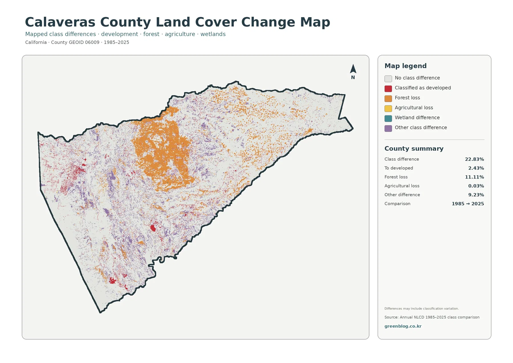
Red pixels representing a change to developed land are much more compact than the broad orange forest-difference area. They appear around several settled locations and along smaller developed corridors. Comparing those red areas with the 2025 impervious map is useful because one map identifies a long-term class change and the other shows the present concentration of hard surface. They answer related but different questions and should not be treated as interchangeable.
Purple “other difference” pixels are distributed through many parts of the county. That category groups changes not separated into the headline classes, so it should not be given one simple environmental explanation. The most reliable reading is spatial: note where the differences cluster, compare them with the current land-cover class, and use a more specialized disturbance or land-management dataset if the reason for change matters.
Water features help organize the west-to-east comparison
Although water occupies only 2.05% of the county, it is one of the easiest classes to use as a geographic reference. Blue reservoirs and water bodies stand out against the tan, light green, and dark green land-cover classes. They make it possible to return to the same location on the forest, impervious, and change maps without relying on road labels or parcel boundaries that are not part of these sheets.
The relationship around those water bodies varies across the county. Western water features are generally surrounded by more open grass and shrub cover, while areas farther east sit closer to forest-dominated landscapes. Developed pixels may appear near some shore or corridor locations, but the maps only show co-location. They do not establish that a water body caused settlement or that the surrounding land has any particular legal use.
Small streams, narrow wetland strips, and shorelines are also subject to raster generalization. A 30-meter grid cannot trace every bank with survey precision, and mixed shoreline cells may be labeled as water, wetland, vegetation, or another dominant class. For watershed education and county-scale comparison the pattern is still useful, but a detailed stream boundary or regulatory wetland question requires a more specialized source.
Choosing the right map and downloading the four JPG files
Start with the full Calaveras County California Land Cover Map when the goal is a broad overview. It places forest, shrubland, grassland, developed land, water, wetlands, and other mapped classes on one sheet. For a classroom or report that needs to explain why the county looks different from west to east, this is the most complete single reference because the major vegetation and settlement patterns can be seen together.
Switch to the forest-and-farmland map when the main question is the contrast between wooded and open landscapes. Use the impervious map for present-day hard surfaces and settlement intensity. The change map belongs beside one of the 2025 maps rather than by itself, because the current cover helps explain what is present today where a historical class difference is shown.
The on-page WebP images are convenient for quick reading, while the original JPG files are better when a larger standalone map is needed for printing, slides, schoolwork, or reference notes. All four JPGs use the same county identity and can be downloaded together, so a project can move from a general overview to a more focused comparison without searching for each map separately.
What to keep in mind before using the maps as evidence
Annual NLCD is designed for consistent land-cover comparison over large areas. It is not a parcel survey, zoning map, ownership map, or development-permit record. Land cover describes the physical surface interpreted from remote-sensing data, while land use and zoning describe how land is used, regulated, or legally designated. Those concepts often overlap in everyday language but should remain separate when making a formal claim.
Scale matters as well. The land-cover products use a 30-meter raster grid, meaning each square cell summarizes an area that can contain multiple materials or vegetation types. Edges between forest and shrubland, narrow roads, shoreline vegetation, and small buildings can be simplified. A class is therefore a useful generalized label, not a guarantee that every square meter inside the cell has the same surface.
Finally, the maps represent specified observation years. The current land-cover and impervious sheets are labeled 2025, while the comparison spans 1985 to 2025. Conditions after those dates may differ, and the long-term comparison can include both real surface change and classification variation. For property decisions, regulatory questions, or a detailed explanation of a particular disturbance, consult current county records and more specialized datasets.
Frequently Asked Questions
Where is forest most concentrated in Calaveras County?
The 2025 map shows the broadest and most continuous forest cover across the eastern and northeastern portion of the county. Shrubland and grassland become more prominent toward the west, with a mixed transition through the center.
Why is mapped agriculture only 0.11% when Calaveras County has ranching and agricultural activity?
The 0.11% value is a land-cover classification, not a measure of the county’s agricultural economy or all land used for agriculture. Grazing land can be mapped as grassland or shrubland because land cover describes the physical surface rather than legal or economic use.
Does the 11.11% forest-loss class prove permanent deforestation from 1985 to 2025?
No. It identifies cells classified as forest in the earlier comparison and as another class in the later one. Real vegetation change may be involved, but recovery stage, disturbance, mixed pixels, and classification variation can also affect the result. Cause and permanence require additional evidence.
Map File Information
The ZIP contains four original JPG maps for Calaveras County: 2025 land cover, forest and farmland, impervious surface and developed land, and 1985–2025 land cover change. Use them for printing, classroom reference, presentations, and county-scale map comparisons.
- Included Files: Use only the versions confirmed in the article and supplied images
- File Type: Use the confirmed download contents
- Intended Use: Printing, education, presentations, and map-based projects
Related Maps
- Alameda County California Land Cover Map
- Alpine County California Land Cover Map
- Amador County California Land Cover Map
Sources and further reading
Land-cover and impervious-surface classes can be checked through the MRLC Annual NLCD Data portal and the USGS Annual NLCD Land Cover Classification documentation. County boundary data and geographic identifiers are available from the U.S. Census Bureau TIGER/Line Shapefiles.
For local context, see the official Calaveras County General Plan and its General Plan Environmental Impact Report, which discuss the county’s western open landscapes and eastern forest setting. The Calaveras County Agriculture Production Reports provide additional local context for agricultural activity that should not be confused with the NLCD agriculture land-cover class.
Green Map creates custom-edited map images using open geographic data sources such as geoBoundaries, Natural Earth, OpenStreetMap, and government open data.
These maps are edited visual materials, not raw data files, and are provided for education, documents, presentations, and graphic reference.