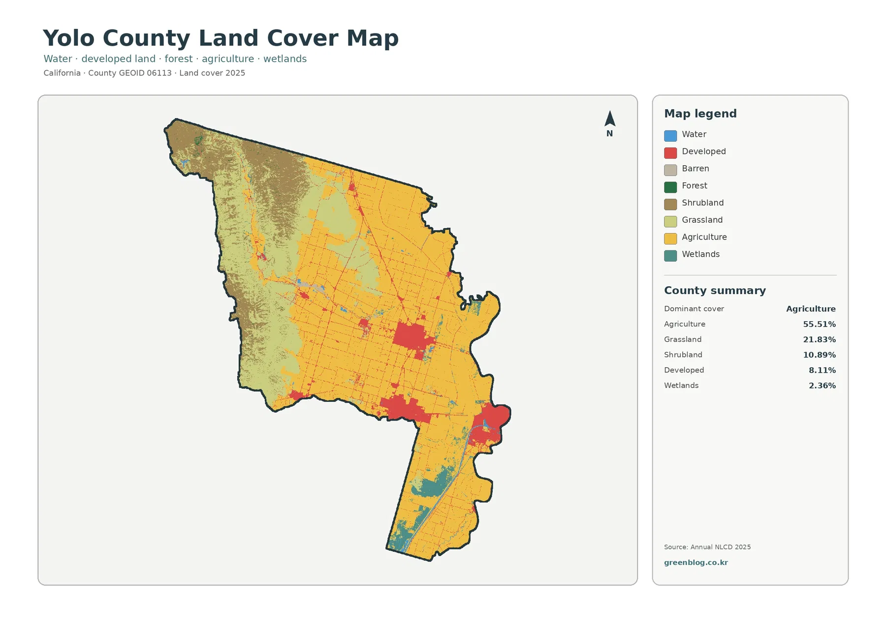
The Yolo County California Land Cover Map is dominated by agriculture at first glance, but the county changes sharply from east to west. Cropland covers much of the central and eastern valley floor, grass and shrub cover expands across the western uplands, and the largest developed patches gather around Woodland, Davis, and West Sacramento. The four maps on this page separate those patterns so the county is easier to understand than it would be from one percentage alone.
The four original JPG maps can be downloaded together in one ZIP near the end of the article. They show 2025 land cover, a simplified forest-and-farmland view, fractional impervious surface, and mapped class differences between 1985 and 2025. Land cover is not the same as zoning, ownership, or legal land use; it is a satellite-based classification of what covers the ground, such as crops, grass, shrubs, wetlands, water, or developed surfaces.
Table of Contents
Agriculture defines the valley, but not the whole county
The 2025 summary assigns 55.51% of Yolo County to agriculture. Grassland accounts for 21.83%, shrubland 10.89%, developed land 8.11%, wetlands 2.36%, water 0.91%, and forest 0.15%. Barren land appears in the legend, but the supplied summary does not list a separate percentage for it, so no unverified value is added here. The leading agricultural share is important, yet the location of each class explains the county far better than the ranking by itself.
Across the central and eastern valley floor, agricultural cover forms a broad, nearly continuous field. The western side looks very different: grassland and shrubland expand as the terrain rises toward the Blue Ridge and Coast Range. Developed land is not spread evenly across the county but forms distinct clusters, while wetlands and water become locally conspicuous in the southeast. These contrasts make Yolo County a useful example of how one countywide percentage can hide several very different landscapes.
| 2025 class | County share |
|---|---|
| Agriculture | 55.51% |
| Grassland | 21.83% |
| Shrubland | 10.89% |
| Developed | 8.11% |
| Wetlands | 2.36% |
| Water | 0.91% |
| Forest | 0.15% |
Yolo County’s General Plan vision describes the Blue Ridge Mountains on the west, the Putah and Cache Creek watersheds, and the Sacramento River and Delta on the east. Those references are not substitutes for the land-cover data, but they provide geographic context for the map. The county’s east-to-west shift from river lowlands and agricultural plains to open uplands is consistent with the broad pattern visible in the supplied image.
The west side changes quickly from cropland to open cover
The forest-and-farmland map simplifies the palette and makes the agricultural footprint especially clear. Cropland spreads around Woodland, continues south toward Davis, and occupies much of the eastern half of the county. Roads, towns, channels, and other surfaces interrupt that field, but the agricultural block remains the dominant mapped feature across the valley.
Move west, however, and the continuous cropland pattern breaks apart. Grass and shrub cover occupies large portions of the uplands, with agriculture extending into selected valleys and flatter areas rather than covering the entire western edge. This is a surface-cover distinction, not a map of agricultural ownership or farmland-protection status. A parcel can be legally agricultural even when the satellite classification for a particular year records a different surface condition.
Forest is only 0.15% in the county summary. That figure should not be read as proof that trees are almost absent. Annual NLCD assigns representative classes to 30-meter raster cells, so narrow riparian tree bands, farm-edge trees, and small groves can be mixed with surrounding cover. The low percentage is better understood as evidence that extensive forest is not the dominant countywide land-cover type.
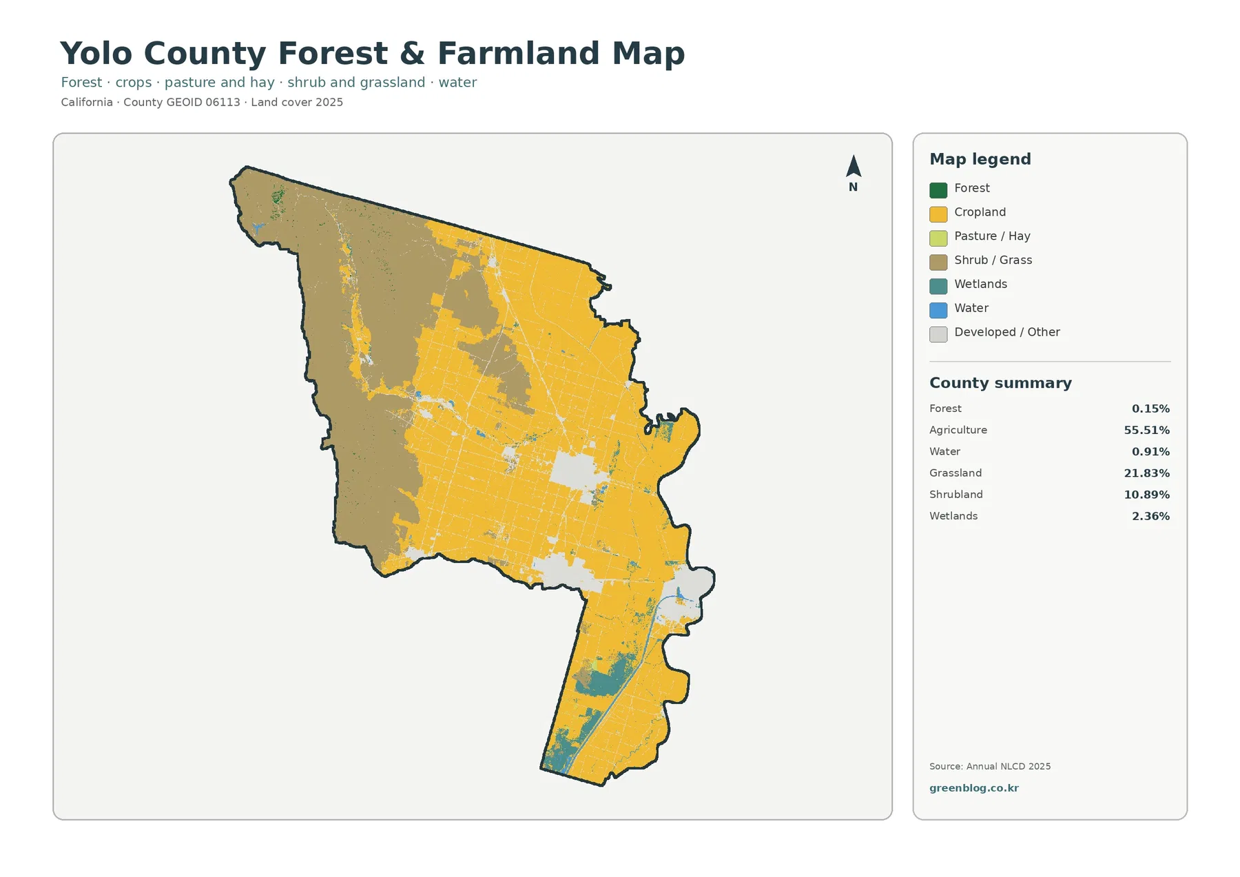
For agricultural presentations, this map gives useful location information that a countywide percentage cannot provide. Showing that the 55.51% agricultural share is concentrated mainly on the valley floor, while western uplands are much more open and non-crop, prevents the misleading impression that the entire county has the same farm landscape. It also helps explain why agricultural, natural, and urban topics need different map views even within one county.
Hard surfaces cluster around three urban centers
Impervious surface measures pavement, rooftops, and other hard surfaces that do not readily absorb water. Yolo County has a mean impervious value of 3.30%, while 3.03% of the mapped area is in cells that are at least 50% impervious. Those numbers are lower than the 8.11% developed-cover share because developed land can include lawns, trees, soil, and other permeable surfaces along with buildings and streets.
The impervious map makes the county’s settlement pattern easy to see. Stronger values concentrate around Woodland, Davis, and West Sacramento. Between those centers, the agricultural plain is mostly light, while roads and smaller settlements appear as thin lines and small patches. West Sacramento stands out sharply on the eastern edge, and Davis and Woodland form two additional compact concentrations separated by large areas of farmland.
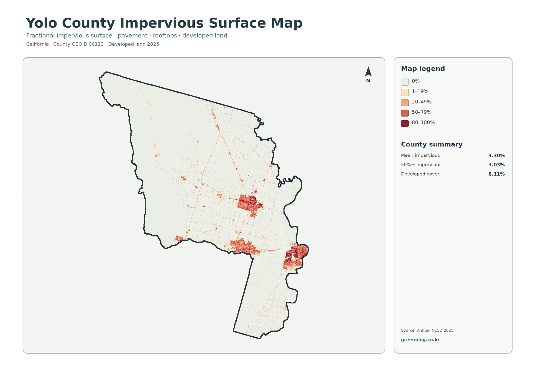
This map is useful for comparing broad urban and rural surface patterns, but it is not a neighborhood drainage map or a parcel-level engineering survey. A 30-meter cell can contain pavement, vegetation, buildings, and bare ground at the same time. Use the county map to identify where hard surfaces are concentrated, then use local engineering, flood, or planning data when a decision depends on conditions at a specific site.
Yolo Bypass makes the southeast look different from the farm belt
The southeastern portion of the county is low and agricultural, yet it does not look identical to the central farm belt. Wetland and water classes become more visible around the Yolo Bypass, where agricultural land, seasonal water, habitat areas, and channels occur close together. Yolo County’s parks information identifies the Yolo Bypass Wildlife Area near Davis and West Sacramento, giving a useful local reference for the wetland concentration shown on the map.
Other water corridors also help explain breaks in the agricultural pattern. The Sacramento River runs along the eastern side, Putah Creek is important near the southern boundary, and Cache Creek crosses the county toward the valley. The county’s Cache Creek Area Plan addresses management and restoration along Lower Cache Creek. These sources do not change the mapped percentages, but they help place the water and wetland colors in a real county setting rather than treating them as isolated map symbols.
Wetlands account for only 2.36% of the countywide summary and water 0.91%, yet those classes can be locally important where they are concentrated. This is why a percentage should always be read with the map. A small countywide share can still form a continuous and recognizable feature in one part of the county, especially in a low-lying floodplain or river corridor.
Reading the 1985–2025 difference map without overclaiming
The change map compares mapped classes in 1985 and 2025. It reports class differences across 18.53% of the county. Areas classified as developed in the later map account for 2.93%, forest loss 1.99%, agricultural loss 2.30%, and other class differences 11.03%. Wetland difference is shown in the legend, but the supplied summary does not provide a separate county percentage, so it is not estimated here.
The spatial pattern is varied. Red developed differences cluster around the main urban areas. Purple “other class difference” and forest-loss colors are widespread in parts of the western uplands, while agricultural-loss and other changes appear more sparsely across the valley. The map therefore does not suggest one single countywide transition. Different kinds of mapped differences occur in urban, agricultural, and open-land settings.
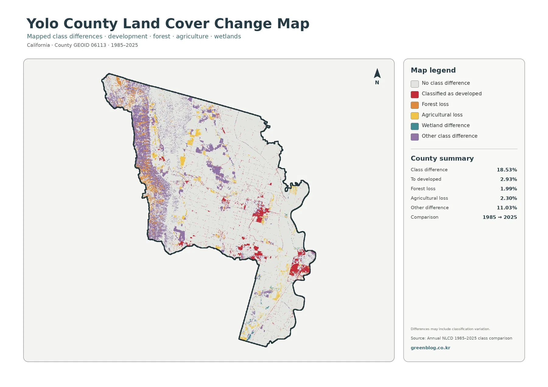
A colored pixel should not automatically be treated as a confirmed real-world conversion. The map itself notes that class differences can include classification variation. Satellite conditions, seasonal timing, and classification methods can differ between observation periods, so some cells can change class without representing a simple on-the-ground conversion. The safest use is to identify places for closer review and then confirm a specific change with historical imagery, planning records, or field information.
The 11.03% “other difference” category is especially important. Folding all of that area into development or agricultural loss would exaggerate what the map actually supports. The comparison is most useful when the legend categories remain separate and the user treats the result as a screening layer rather than a complete history of land-use change.
Which map works best for each task
Start with the general land-cover map when the goal is to understand the county as a whole. It shows the relationship among agriculture, grassland, shrubland, developed land, wetlands, and water in one view. If the question is specifically about the extent of farming, the forest-and-farmland map strips away some detail and makes the agricultural block across the valley easier to follow.
For urbanization or runoff context, the impervious map is the more direct choice because it separates the concentration of hard surfaces from the broader developed-land category. Woodland, Davis, and West Sacramento become immediately visible against the light rural background. For watershed or environmental education, the general map can be paired with the impervious map to contrast Yolo Bypass wetlands and river lowlands with the nearby urban areas and the surrounding agricultural plain.
Use the 1985–2025 comparison when the question is where mapped classes differ over time, not when the question is simply what the county looks like today. Placing it beside the 2025 map helps distinguish current cover from historical classification differences. In presentations or classroom materials, label the observation years and explain that the change layer can include classification variation so the audience does not interpret every colored cell as a confirmed conversion.
Download the four original JPG maps
The ZIP contains four original JPG files: general land cover, forest and farmland, impervious/developed land, and land-cover change. Each image is 2480×1754 pixels and keeps the dimensions of the supplied original asset. The manifest does not mark these files as meeting the project’s A3 high-resolution reference, so the actual pixel dimensions are stated instead of describing them as A3-ready. You can choose the map that best fits a document, class handout, presentation, or county-scale comparison.
Limits of county-scale land-cover data
Annual NLCD is a raster product derived from satellite imagery. The Collection 1.2 material referenced by the package uses 30-meter spatial resolution, so the landscape is represented as grid cells rather than legal parcel polygons. A single cell can contain a field edge, road, trees, buildings, or a narrow channel, and the assigned class generalizes that mixture into a mapped condition.
That scale works well for county and regional patterns, but it cannot replace parcel surveys, zoning maps, wetland delineations, flood maps, or site engineering. Boundaries between agriculture and development can appear cleaner than they are on the ground, and narrow riparian vegetation can be absorbed into adjacent classes. The fractional impervious values are also satellite-based estimates rather than measurements made at every property.
The 2025 maps represent a particular observation and classification period. Crops rotate, fields may be fallowed, habitat restoration changes vegetation, floods alter wetland appearance, and new development can occur after the mapped year. When a project depends on current site conditions, use these county maps for geographic context and then check more recent imagery or the appropriate county, city, state, or federal record.
Frequently Asked Questions
Where is Yolo County’s agricultural cover most concentrated?
Agriculture accounts for 55.51% of the 2025 summary and is concentrated mainly across the central and eastern valley floor. The western uplands contain much more grassland and shrubland, so the agricultural share should not be interpreted as an even blanket across the entire county.
Why is developed cover 8.11% but mean impervious surface only 3.30%?
They measure different things. Developed land is a broad land-cover class that can include lawns, trees, bare soil, and other permeable surfaces around buildings. Impervious surface measures the fraction covered by hard surfaces such as pavement and rooftops, so the two countywide percentages are not expected to match.
Does every colored cell on the 1985–2025 map represent a confirmed land conversion?
No. The comparison shows mapped class differences, and the map notes that classification variation can be included. A specific development, agricultural loss, or vegetation change should be confirmed with historical imagery, planning documents, field information, or another time-consistent source.
Map File Information
Download the four original Yolo County land-cover JPG maps together in one ZIP file.
- Printable Size: 2480×1754 pixels each
- File Type: ZIP containing 4 JPG files
Related Maps
- Alameda County California Land Cover Map
- Alpine County California Land Cover Map
- Amador County California Land Cover Map
Sources and further reading
The percentages and spatial observations in this article follow the supplied 2025 Yolo County land-cover maps and the 1985–2025 class comparison. These official sources provide definitions for the data and county-specific context for agriculture, watersheds, and natural areas.
- MRLC Annual NLCD Data – official access to Annual NLCD products
- USGS Annual NLCD Land Cover Classification – land-cover classes and product documentation
- Yolo County General Plan Vision Statement – county context for Blue Ridge, Putah and Cache Creeks, the Sacramento River, and the Delta
- Yolo County Cache Creek Area Plan – Lower Cache Creek management and restoration context
- Yolo County Parks Hiking – references for Yolo Bypass Wildlife Area and Putah Creek
- Yolo County Agriculture – official county agricultural department information
Green Map creates custom-edited map images using open geographic data sources such as geoBoundaries, Natural Earth, OpenStreetMap, and government open data.
These maps are edited visual materials, not raw data files, and are provided for education, documents, presentations, and graphic reference.