Roberts County sits in the northeastern Texas Panhandle, and its maps show a county with two very different visual anchors. Miami, the county seat, is concentrated near the southeastern edge where U.S. 60 and U.S. 283 provide clear road references. Farther north, the landscape is dominated less by towns than by the broad Canadian River valley and a dense network of smaller creeks. The maps on this page are designed to make those relationships easy to follow, and the same four subjects are available as high-resolution A3 JPG files in the downloadable ZIP.
A useful way to begin is with Miami rather than the geometric center of the county. Miami is not centrally placed; it lies toward the southeast, with U.S. 60 running through the area and U.S. 283 extending northward into the county. Once that location is fixed, the other layers become easier to compare. The city map emphasizes how isolated the main settlement appears within a large county, the terrain-and-water map shifts attention to river valleys, and the elevation layer explains why northern Roberts County looks so different from the higher ground across much of the south and southwest.
Table of Contents
Miami and the numbered highways provide the quickest geographic reference
The general county map gives the most complete first look at Roberts County because it combines the boundary with roads, waterways, and named places. Miami is the clearest settlement label and sits close to the southeastern side of the county. U.S. 60 passes through the Miami area, while U.S. 283 runs north from near the city and becomes an easy reference for following the county from south to north. Other numbered roads, including routes marked 70, 748, and 16, add useful orientation around the southern and northern parts of the map.
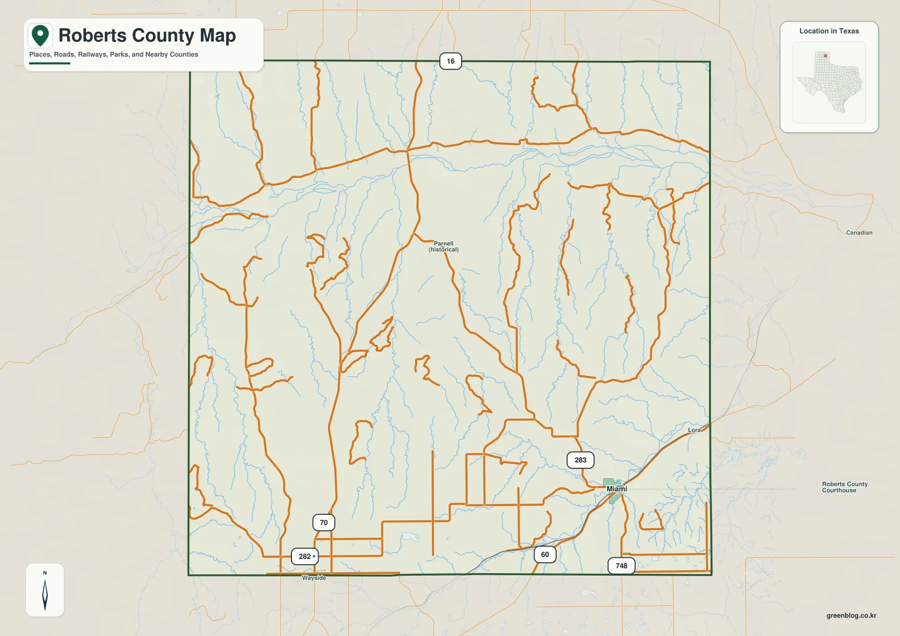
Parnell (historical) is labeled closer to the middle of the county, which helps distinguish a historic place name from the present-day county seat. Outside the boundary, labels such as Canadian, Lora, and Wayside give additional context for judging where the county ends. These surrounding references are especially useful because Miami is so far from the center. A reader who starts with the city and then traces the county outline can quickly see how much land extends north and west beyond the main settlement.
The road pattern also changes as the eye moves away from Miami. Southern routes include long straight segments that are easy to follow, but the central and northern parts contain many bends and interruptions around stream valleys. The blue drainage lines on the general map hint at the reason. Roberts County is not simply a flat rectangle covered by a regular road grid; many roads share the landscape with narrow valleys that cut through the interior. The terrain-and-water layer makes that relationship much clearer.
The city layer shows how strongly settlement is concentrated toward the southeast
The supplied city map has a deliberately simple message. Its ranked city index identifies Miami as the single major city on the layer, and the marker appears near the southeastern edge of Roberts County. That arrangement says more than a longer list of small place names would. The county covers a large area, yet its principal mapped settlement is concentrated near one corner, leaving a broad northern and western interior without comparable city markers.
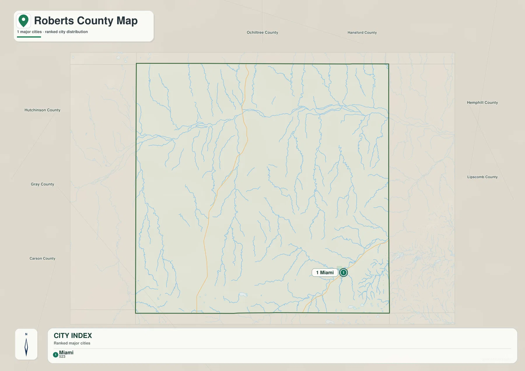
County names around the map help establish direction even though the layer itself stays uncluttered. Ochiltree County and Hansford County appear to the north, Hutchinson County is shown to the west, and Hemphill County and Lipscomb County appear on the eastern side. Gray County and Carson County are visible farther south and southwest. These labels make Miami’s position easier to judge and reinforce the fact that the settlement lies much closer to the eastern and southern sides of Roberts County than to the far northwestern interior.
This is why the city layer works best as an orientation tool rather than as a detailed street map. After locating Miami here, it is easy to return to the general map and find U.S. 60 and U.S. 283. From there, the water and elevation layers add the natural setting around the same southeastern location. That sequence turns the city marker into a fixed reference point for comparing every other map in the set.
The Canadian River defines the north, while smaller creeks divide the interior
The terrain-and-water map shifts attention away from roads and toward the shape of the land. The Canadian River is the dominant feature, crossing northern Roberts County from west to east through a broad valley. Shaded relief makes the valley visible even before individual stream labels are read. The river corridor is wide enough to form a major geographic division across the county, and numerous smaller drainages descend toward or away from that northern system.
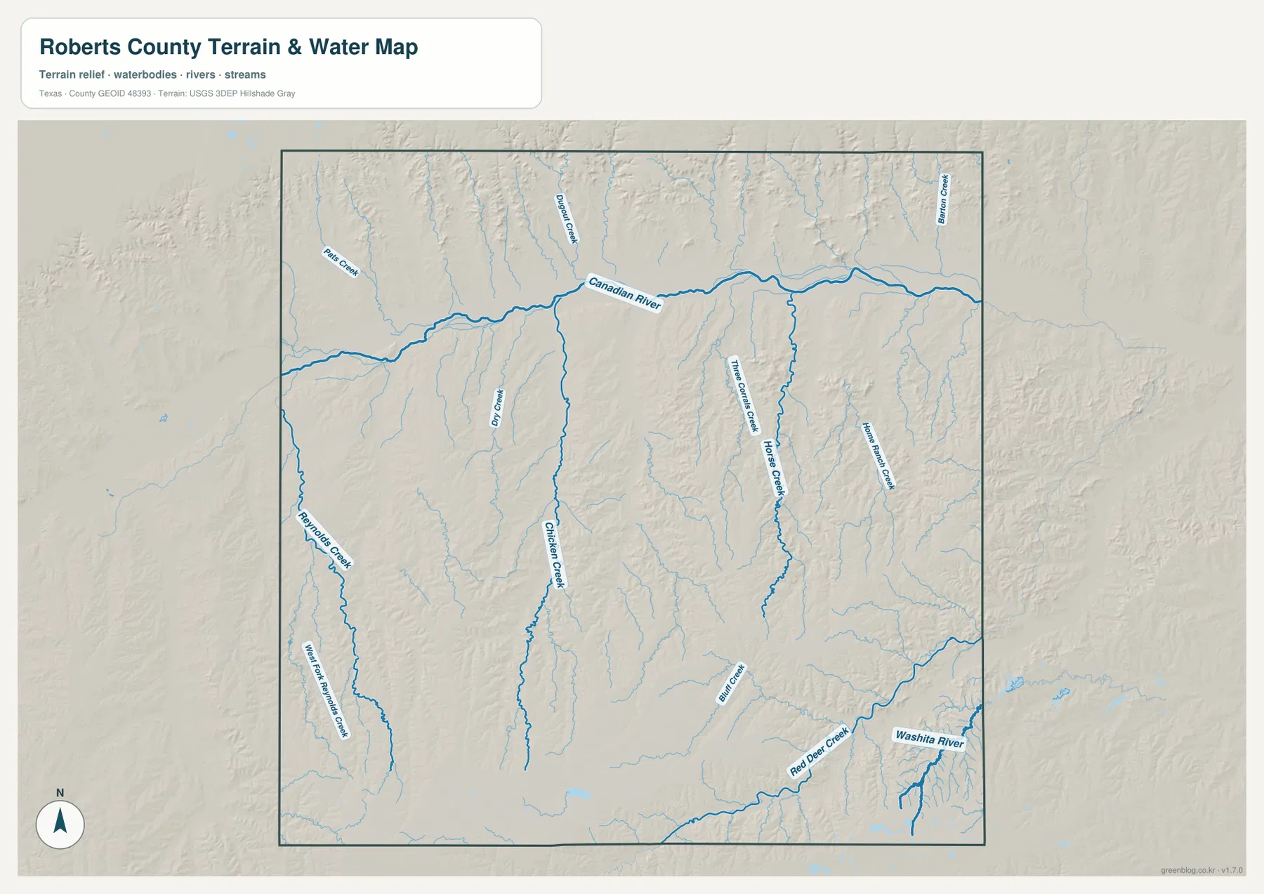
South of the Canadian River, Dry Creek and Chicken Creek extend through the western and central parts of the county. Farther east, Three Corner Creek and Horse Creek occupy long narrow valleys, with Home Ranch Creek visible beyond them. These channels are easier to understand when the labels are viewed together with the shaded terrain. They are not isolated blue lines on a flat background; each follows lower ground between ridges, creating a repeated pattern of narrow valleys through the central county.
The southeastern drainage is separate enough to deserve its own look. Bluff Creek and Red Deer Creek appear closer to the Miami side of the county, while the Washita River is labeled near the southeastern edge. Comparing these features with the Canadian River prevents the common mistake of treating all of Roberts County as one simple north-flowing drainage area. The map shows several distinct valleys, and the southeastern waterways give Miami a local terrain context that is easy to miss on the city layer alone.
This layer is intended for geographic reference, not for determining a parcel’s flood status, legal water boundary, water rights, or engineering conditions. Those questions require specialized official sources. For the purposes of this page, the important information is the location of the named rivers and creeks and the way their valleys shape the broad county landscape.
Elevation makes the Canadian River lowlands stand out against the higher south
The supplied elevation map reports an actual range of about 724 to 994 meters and a mean elevation of about 863 meters. Its strongest contrast runs across the north. The Canadian River corridor appears as a broad dark-green band, marking some of the lowest continuous terrain in the county, while large areas of the south and southwest shift into tan and brown colors that represent higher ground. The result is a clear county-scale distinction between the river lowlands and the elevated southern interior.
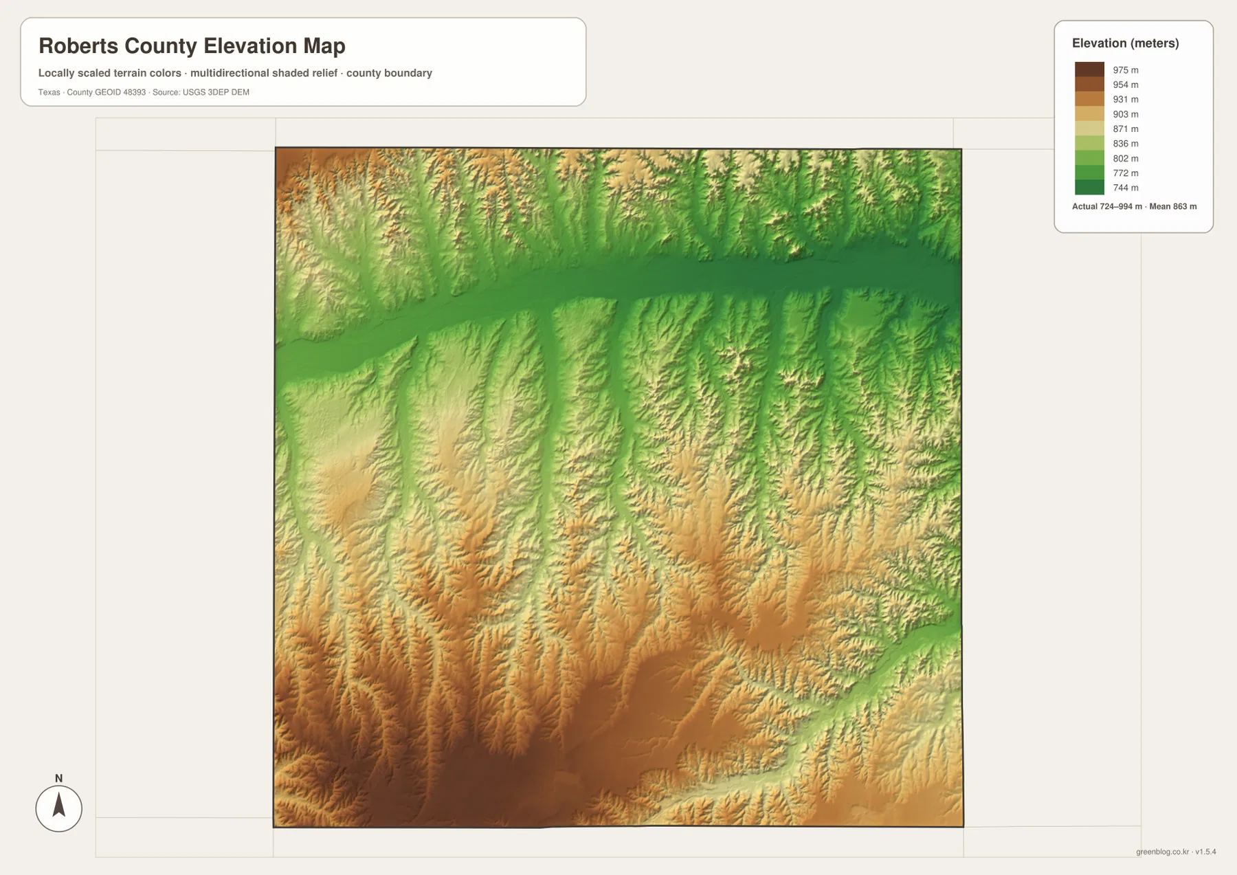
The change is not a smooth north-to-south slope. Narrow green valleys extend southward from the Canadian River corridor and cut into higher terrain, often following directions similar to the creeks shown on the water map. That gives central Roberts County a more broken surface than a simple color gradient would suggest. Higher ridges and plateaus are repeatedly interrupted by drainage valleys, which is also why some roads on the general map bend rather than continuing in a perfect grid.
The southeast shows the same relationship on a smaller scale. Lower corridors associated with Red Deer Creek and the Washita River are visible against nearby higher ground, so the area around Miami should not be pictured as uniformly level. The Canadian River remains the most dramatic low feature, but it is part of a broader pattern in which watercourses occupy lower terrain throughout the county.
The elevation values are appropriate for broad comparison, not for survey-grade work at a specific property. A building project, drainage plan, legal survey, or other site-specific task would need more detailed elevation information. Here, the map is most useful for understanding the relative height difference between the Canadian River valley, the higher southern and southwestern areas, and the smaller drainage cuts that cross them.
Following the same location across the maps explains the county more clearly
The four supplied maps are most useful when treated as views of the same places rather than as separate illustrations. Start with Miami and U.S. 60 on the general map, then follow U.S. 283 north to establish the county’s orientation. Move to the water layer and the Canadian River becomes the main northern landmark. Open the elevation layer and the same corridor turns into a broad low band. The information changes from roads to water to height, but the geography stays fixed, which makes the differences easy to connect.
Northern roads provide a good example. On the general map, some routes curve or change direction instead of forming a regular grid. The terrain-and-water map shows the Canadian River and numerous tributary valleys in the same area, while the elevation map reveals low corridors cutting through higher ground. Looking at these layers together makes the road pattern more understandable without inventing a separate explanation for every bend.
Miami can be compared in the opposite order. The city map first establishes its southeastern location. The general map then adds U.S. 60, U.S. 283, nearby roads, and stream lines. The water map shows Red Deer Creek and the Washita River in the same general part of the county, and the elevation layer places those valleys within a landscape that rises across much of the south and southwest. This cross-map approach gives Miami a much richer setting than any single layer can provide.
Choose the first map according to the question you need to answer
For boundaries, named places, and highway orientation, the general county map is the fastest starting point. It keeps Miami, Parnell (historical), U.S. 60, U.S. 283, other numbered roads, streams, and the county outline together. If the main goal is simply to see where the principal mapped city sits within the county, the city index is cleaner and makes Miami’s southeastern position immediately obvious.
For the natural landscape, the terrain-and-water map is more informative. It labels the Canadian River along with Dry Creek, Chicken Creek, Three Corner Creek, Horse Creek, Home Ranch Creek, Bluff Creek, Red Deer Creek, and the Washita River. When relative height matters more than names, the elevation map is the clearest choice because the low northern corridor and higher southern areas are visible at a glance. Switching between these layers lets the reader select detail according to the task instead of forcing every feature onto one crowded image.
The images embedded on the page are convenient for quick reference, while the downloadable files are better for printing or close offline viewing. The ZIP contains high-resolution A3 JPG versions of the county map, city map, terrain-and-water map, and elevation map. A practical workflow is to use the page to identify which map contains the information you need, then open the matching larger JPG when small road labels, creek names, or relief details deserve a closer look.
Frequently Asked Questions
Where is Miami located within Roberts County?
Miami is shown in the southeastern part of Roberts County. On the general map it is easy to locate near U.S. 60 and U.S. 283, while the city index emphasizes how close the main settlement is to the county’s southeastern edge rather than its center.
Why is the Canadian River corridor so low on the elevation map?
The Canadian River occupies a broad valley across northern Roberts County. The terrain-and-water map shows that valley together with several tributary drainages, and the elevation layer marks the same corridor in dark green as one of the county’s lowest continuous areas.
What elevation range is shown for Roberts County?
The supplied elevation map states an actual range of about 724 to 994 meters and a mean of about 863 meters. Those values describe county-scale terrain and are useful for broad comparison, but they are not a substitute for survey-grade measurements at a specific site.
Sources and reference data
Boundary and road data can be checked through the U.S. Census Bureau TIGER/Line Shapefiles. Waterway reference data are available from USGS National Hydrography, and elevation data can be compared with the USGS 3D Elevation Program. The descriptions of Miami, the Canadian River, named creeks, roads, and the 724–994 meter elevation range on this page are based on the Roberts County maps and asset manifest supplied in the rewrite package.
Map File Information
The ZIP contains high-resolution A3 JPG versions of the Roberts County general map, city map, terrain and water map, and elevation map. The larger files are suitable for printing, classroom materials, presentations, and detailed offline reference.
- Included Files: County map, city map, terrain and water map, elevation map
- File Type: High-resolution A3 JPG
- Intended Use: Printing, education, presentations, and map reference
Related Maps
Green Map creates custom-edited map images using open geographic data sources such as geoBoundaries, Natural Earth, OpenStreetMap, and government open data.
These maps are edited visual materials, not raw data files, and are provided for education, documents, presentations, and graphic reference.