Mohave County Arizona Land Cover Map — 88.08% Shrubland, River-Edge Development, and 1985–2025 Change

Mohave County occupies a large part of northwestern Arizona, where broad desert landscapes meet the Colorado River, reservoir shorelines, scattered mountain forests, and several separated population centers. The 2025 land-cover summary is unusually clear: shrubland covers 88.08% of the county, while forest accounts for 7.00%. Developed land is only 1.11%, so built surfaces appear as small concentrations against a very large undeveloped background rather than as one continuous urban area.

This page compares four views of that landscape: current land cover, forest and farmland, developed land, and mapped class differences from 1985 to 2025. The four original JPG maps are available together in one download, while the WebP images in the article are lighter previews for on-screen reading. The maps are useful for county-scale reference, environmental education, presentations, and broad comparisons, but they do not show zoning, parcel ownership, or legal land-use rights.

Development stands out because most of the county is not developed

The developed-land view removes most of the land-cover colors and isolates the places where buildings, paved surfaces, and other developed classes are present. Only 1.11% of Mohave County is summarized as developed in 2025. On a county this large, that small percentage matters less than its location. The strongest clusters lie along the western and southwestern side of the county, with another important concentration farther inland around the Kingman area and smaller scattered developed patches elsewhere.

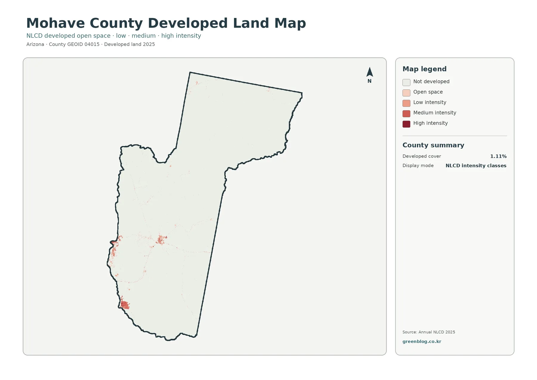
The county’s current General Plan uses planning areas such as the Bullhead City vicinity, Golden Valley vicinity, Kingman vicinity, Lake Havasu City vicinity, and the Arizona Strip. Those official place references help orient the clusters visible on the map. Developed areas near the Colorado River and Lake Havasu side of the county can be read alongside Bullhead City and Lake Havasu City, while the larger inland patch provides context for Kingman. The map shows spatial association, not proof that any single road, plan, or water source caused the development.

The legend separates developed open space from low-, medium-, and high-intensity development. These classes describe the amount of built and impervious surface within a raster cell. A residential neighborhood with substantial vegetation can fall into a lower-intensity class, while denser commercial or urban surfaces can appear in higher-intensity classes. Because these are land-surface categories rather than municipal boundaries, several intensities can occur within the same city and thin transportation features may be simplified at county scale.

Shrubland defines the broad county landscape

The general land-cover map puts the developed clusters back into their larger setting. Shrubland covers 88.08%, making it by far the dominant class. Forest is second at 7.00%, followed by grassland at 1.76%, developed land at 1.11%, barren land at 0.76%, water at 0.63%, wetlands at 0.43%, and agriculture at 0.23%. Together, these values describe a county where most land has a dry shrub-dominated surface and the other classes occur in much smaller, more localized areas.

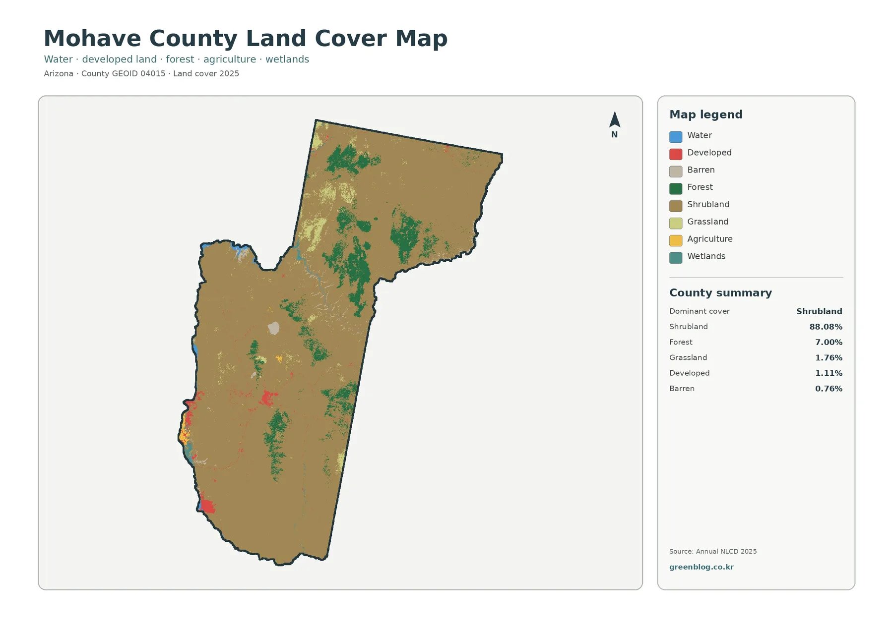
The forest class does not form one continuous block. Green patches are scattered across northern, central, and southern uplands, creating sharp local contrasts with the surrounding shrubland. Water is mostly confined to the western side and reservoir areas, while developed colors are concentrated near population centers. Agriculture is too limited to dominate the county view, but small agricultural areas are visible near the lower Colorado River side of the county. This mix is easier to understand spatially than by percentages alone.

Land cover describes what is physically covering the ground in the classified imagery. It should not be read as a zoning map. A cell classified as shrubland may be public, tribal, state, or private land, and a developed cell can contain many different legal uses. The map is best for questions such as where vegetation types are broadly concentrated, how developed areas compare with the surrounding desert, and where water or forest classes interrupt the dominant shrubland surface.

Forest and agricultural classes occupy small but meaningful areas

The forest-and-farmland view reduces the visual competition from other classes and makes the smaller vegetation categories easier to locate. Forest remains 7.00%, while agriculture is only 0.23%. Grassland accounts for 1.76%, water for 0.63%, wetlands for 0.43%, and shrubland for 88.08%. The result is not a conventional farm map: it is a desert county map in which forests and agricultural land appear as relatively small exceptions to the much larger shrub and grass background.

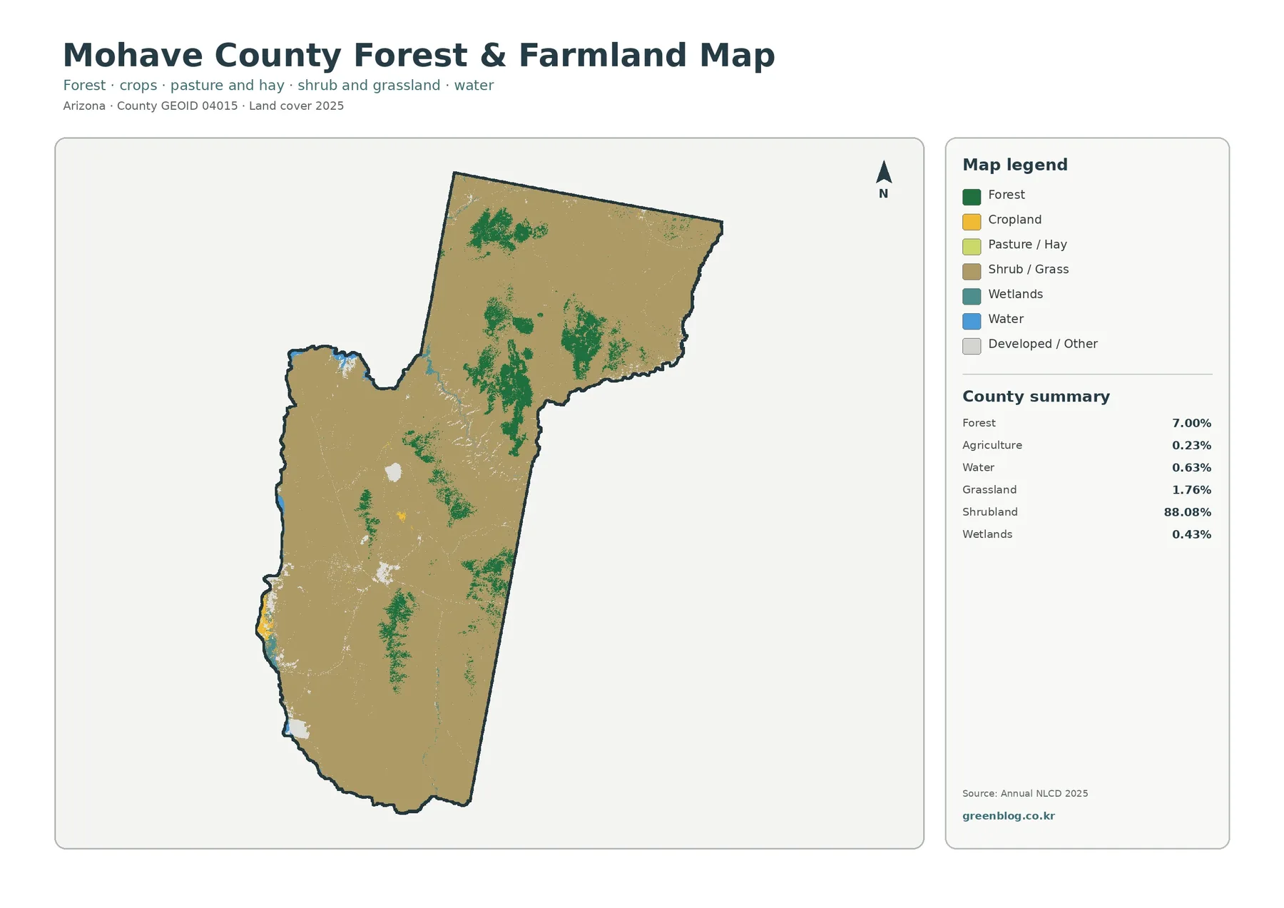
The forest patches are especially useful for understanding how varied the county can be with elevation. The Bureau of Land Management describes Wabayuma Peak Wilderness, about 20 miles southeast of Kingman, as having lower Sonoran and Mohave Desert vegetation, Arizona chaparral at higher elevations, and ponderosa pine on mountain summits. That official description does not identify every green cell on this county map, but it provides a concrete example of why forest can occur as isolated upland patches within a predominantly desert county.

Agricultural colors are sparse, with the most noticeable concentration near the southwestern Colorado River side. That pattern should be read cautiously: 0.23% is the classified agricultural surface, not a measure of the economic value of agriculture or the number of farms. Water and wetlands are similarly small by area, yet their location along the river and reservoirs is important for understanding the western edge of the county. A small percentage can still mark a feature that is locally significant.

The Colorado River and reservoirs explain why the western edge looks different

Mohave County’s 2025 General Plan describes the Colorado River as the county’s primary source of water for urban and agricultural use and identifies Lakes Mead, Mohave, and Havasu as important water and recreation resources. On the land-cover maps, blue water cells form a narrow part of the county’s total area, but they sit next to some of its most visible developed concentrations. The western edge therefore looks very different from the broad interior shrubland, even though water itself represents only 0.63% of the mapped county area.

Wetlands account for 0.43% and appear in small, narrow areas rather than broad expanses. Their proximity to water can be useful for watershed or habitat discussions, but the 30-meter classification is too generalized for wetland permitting or boundary decisions. For those purposes, current agency wetland inventories, field information, and regulatory maps are required. The land-cover map instead provides a county-wide frame for seeing where wet surfaces occur relative to desert vegetation and development.

This west-to-interior contrast is one of the most useful ways to read the set. Near the river and reservoirs, water, developed surfaces, wetlands, and small agricultural areas occur close together. Farther inland, shrubland dominates for long distances, interrupted by forest patches and isolated communities. The northern Arizona Strip section adds another large area where shrubland and upland vegetation can be compared with the more populated western and southern parts of the county.

Most cells did not change class between 1985 and 2025

The change map compares the 1985 and 2025 classifications. A total of 3.58% of the county is marked with a class difference, which means more than 96% remains in the no-class-difference background on this comparison. The summary reports 0.49% changed to developed, 0.42% forest loss, 0.06% agricultural loss, and 2.46% other class differences. The legend also contains a wetland-difference category, but the summary panel does not give a separate percentage for it, so no value is inferred here. This distinction matters because the map is not simply a development-growth map.

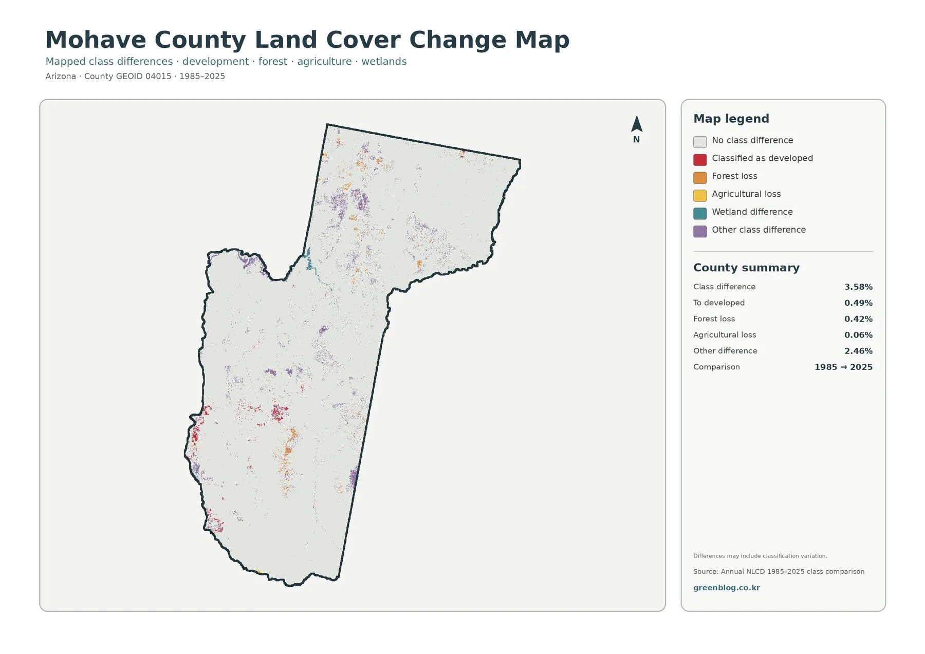
Red developed-change patches are more noticeable around parts of the western and southwestern developed areas, while other change colors occur as smaller clusters across the county. Forest-loss colors appear in limited upland areas rather than as a county-wide band. The visual balance matters: the change colors can look prominent because they sit on a pale background, but they still represent a small fraction of Mohave County’s total area. Reading the percentage beside the spatial pattern prevents a few bright patches from being mistaken for wholesale county-wide conversion.

The change layer also requires a methodological caution. Differences between two classified raster dates can include classification variability, mixed pixels, and other effects in addition to real ground change. MRLC warns that products from different NLCD release systems should not be mixed casually because methodology differences can appear as change. The map supplied here is a packaged 1985-to-2025 comparison, so it is appropriate for broad location and pattern questions, not for assigning a precise cause or date to a change on an individual property.

A practical way to compare the four map views

Start with the general map when you need to identify the current class at a broad location. It gives the full context: shrubland, forest, grassland, developed land, barren ground, agriculture, water, and wetlands. Once a location is found, switch to the forest-and-farmland view if vegetation or agricultural land is the main question. The reduced legend makes small forest, farm, water, and wetland areas easier to pick out without losing the dominant shrubland background.

For cities and built surfaces, the developed-land map is more efficient because it removes most natural-cover colors. A western river community that occupies only a small part of the county can be difficult to compare on the general map, but the developed-only view makes its extent and intensity classes easier to see. The same technique works for Kingman and smaller developed pockets. Compare locations rather than trying to rank communities by the apparent darkness of a few cells.

Then use the change map as a final layer rather than a starting point. A current developed patch and a red “to developed” change patch answer different questions: one describes the 2025 surface, while the other indicates a class difference between the two comparison years. Likewise, a current forest patch does not necessarily imply forest gain, and a forest-loss mark does not mean the entire surrounding mountain lost forest. Keeping current condition and long-term difference separate avoids many common misreadings.

For a classroom or presentation, a useful sequence is to show the current map first, ask where the dominant shrubland is interrupted, then use the specialized maps to explain those exceptions. Water and development on the west side, forest in upland patches, and small agricultural areas each become easier to discuss in that order. For environmental planning or local research, these maps can provide background context before moving to parcel data, official zoning, watershed studies, or field observations.

Download the four original JPG maps

The download contains one original JPG for each view used on this page. The general map is the best single-file overview, the forest-and-farmland map emphasizes vegetation and small agricultural areas, the developed-land map isolates built surfaces and development intensity, and the change map compares 1985 with 2025. Keeping all four files together makes it easier to move from current condition to a specialized topic without relying on screenshots from the article.

Each source JPG in the package is 2480 × 1754 pixels. The manager keeps those originals rather than artificially enlarging them to claim a higher resolution. For printing, check the target size and make a test print if small legend text is important. For slide decks and documents, preserving the image aspect ratio usually produces a cleaner result than stretching the file to fill a fixed frame.

If you plan to add labels, routes, study areas, or notes, keep a copy of the original and edit a duplicate. Any added parcel, road, ownership, or planning information should come from an authoritative source appropriate to that subject. These land-cover maps show classified surface cover and are not substitutes for surveys, assessor records, zoning maps, engineering plans, or site-specific environmental delineations.

Scale, classification, and date limits matter

Annual NLCD is a raster product derived from Landsat imagery at 30-meter resolution, according to the U.S. Geological Survey. In plain terms, the landscape is divided into 30-meter cells and each cell receives a classification. Narrow roads, small water channels, scattered houses, and sharp vegetation edges can therefore look simplified. A mixed cell containing more than one surface type still has to be represented within the classification system.

That generalization is a limitation for site work but a strength for county-wide comparison. Mohave County is large enough that a parcel-level display would be visually overwhelming. At 30 meters, the maps clearly communicate the broad dominance of shrubland, the limited and clustered developed footprint, isolated forest patches, and the narrow western water features. The maps become less reliable as the question becomes more precise, such as the exact edge of a wetland or the surface material on a single lot.

The current maps represent 2025 classifications. Construction, fire, vegetation recovery, shoreline changes, or other events after that observation period will not appear until reflected in later data. The 1985–2025 change image also summarizes the difference between those dates rather than narrating every intermediate year. Annual products can be consulted when the timing of a particular land-cover shift matters.

Finally, land cover and land use are related but different ideas. Land cover describes the visible surface—shrub, forest, water, developed material, and similar classes. Land use describes how people use or regulate a place, which can involve planning designations, ownership, leases, agriculture, recreation, conservation, or infrastructure. Mohave County Planning & Zoning and other official agencies should be consulted when the question is legal or administrative rather than visual land cover.

Frequently Asked Questions

Related Maps

• Apache County Arizona Land Cover Map
• Cochise County Arizona Land Cover Map
• Coconino County Arizona Land Cover Map

Sources and reference material

MRLC Annual NLCD Data provides official U.S. land-cover and land-change products and access information for the dataset family used to interpret these classifications.

USGS Annual NLCD Land Cover Classification explains the meaning of land-cover classes such as developed land, forest, shrubland, grassland, agriculture, wetlands, and water.

USGS guidance on Annual NLCD spatial resolution states that the raster data are derived from Landsat imagery at 30-meter resolution.

Mohave County General Plan provides official county planning context, including the Arizona Strip, Bullhead City, Golden Valley, Kingman, and Lake Havasu City vicinity areas.

Bureau of Land Management: Wabayuma Peak Wilderness describes the elevation-driven transition from desert vegetation to chaparral and ponderosa pine in a Mohave County mountain landscape southeast of Kingman.

U.S. Census Bureau TIGER/Line Shapefiles provide official geographic boundary data for counties and other mapped units.