Coconino County Arizona Land Cover Map: Shrub Plateau, Flagstaff Forest, and Sparse Hard Surface

The Coconino County Arizona Land Cover Map makes the county’s scale easier to understand by showing how a tiny built footprint sits inside a much larger shrub-and-forest landscape. Shrubland accounts for 71.51% of the 2025 summary and forest for 23.70%, while the strongest concentration of hard surfaces appears around the south-central Flagstaff area. The contrast between that compact developed cluster and the broad open county is one of the most useful patterns in the set.

Four page previews are included: general land cover, forest and farmland, impervious surface/developed land, and a 1985–2025 change comparison. The four original 2480 × 1754 JPG files are available together in one ZIP from the download section. They work well for county-scale reference, classroom discussion, presentation graphics, and environmental comparison, but they do not replace parcel, zoning, ownership, engineering, or current site-condition records.

Start with the hard-surface map to see how concentrated settlement is

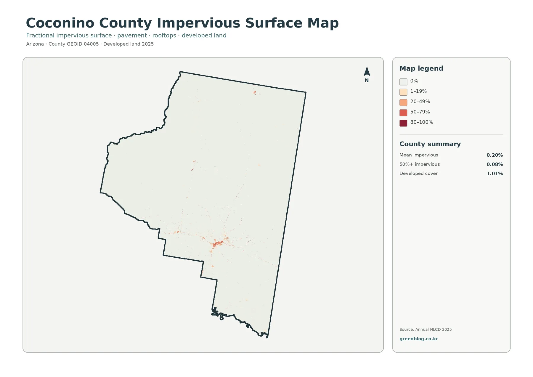
Most of the impervious-surface map is nearly white, which is a strong visual result in itself. Hard surfaces are not spread evenly across Coconino County. The clearest orange and red cluster appears in the south-central part of the county around Flagstaff, with much smaller marks elsewhere. A countywide mean of only 0.20% can therefore coexist with a locally obvious urban center because pavement and rooftops are concentrated rather than evenly distributed.

Impervious surface refers to hard materials such as pavement and roofs that limit water infiltration. It is not the same measure as the 1.01% developed land-cover class. A developed classification can include soil, trees, lawns, and other permeable surfaces within a settlement. The 0.08% statistic for cells that are at least 50% impervious is narrower again. Keeping all three numbers separate prevents the common mistake of assuming that every area labeled developed is mostly concrete or asphalt.

This map is useful when the question is where built surfaces are concentrated at county scale. It is not precise enough to measure the paved share of a specific parcel, street, campus, or parking lot. A roughly 30-meter classification cell can contain a mix of buildings, road surface, trees, and bare ground, so detailed planning work requires finer imagery and local records.

Shrubland dominates the county, while forest collects in distinct zones

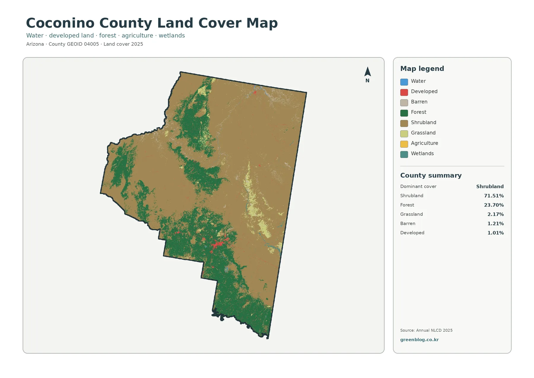
The general land-cover view explains why a single countywide percentage is not enough. Brown shrubland covers a very large share of the east and northeast and also extends across large western areas. Forest is far less extensive overall, yet it forms visually coherent zones rather than a uniform scatter. A north-central band and broader south-central to southwestern forest areas interrupt the shrub-dominated landscape and create some of the strongest internal contrasts on the map.

Grassland at 2.17%, barren land at 1.21%, and developed cover at 1.01% are much smaller shares. Their importance depends on location as much as on percentage. A small developed class can still define the county’s main population center, while barren or grass classes can be locally visible even though they contribute little to the countywide total. Reading the legend together with the map prevents a small number from being dismissed as geographically unimportant.

Land cover describes what the ground surface is classified as, not who owns it or how it is legally zoned. A shrubland cell may lie on federal, tribal, state, county, or private land, and a forest cell is not automatically inside a national forest boundary. Ownership, management jurisdiction, and development permission require separate official sources. That distinction is especially important in a county with large public and tribal landscapes.

The forest-and-farmland view emphasizes forest geography, not farming acreage

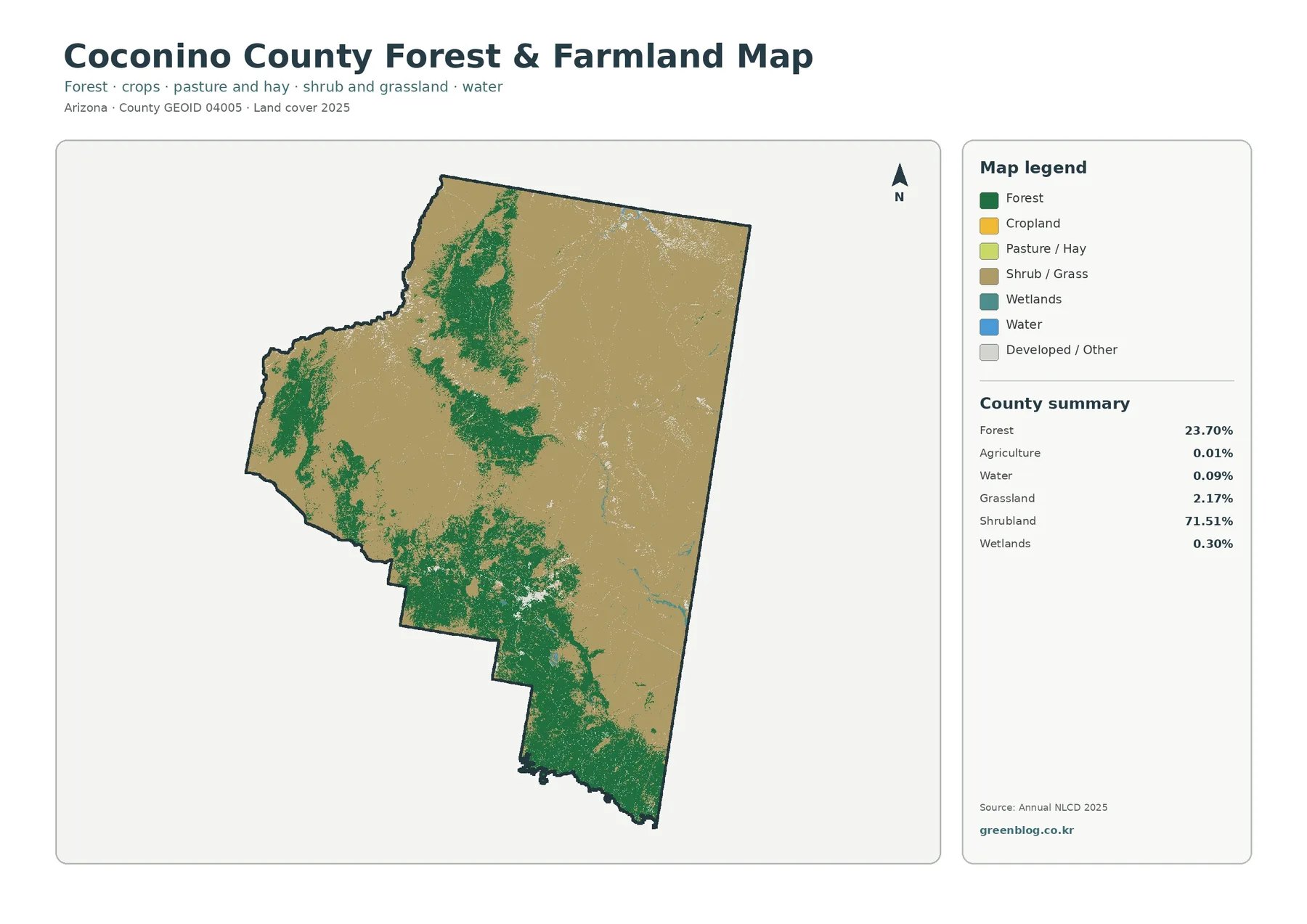
Simplifying the legend makes the location of forest easier to compare. The north-central forest zone is relatively elongated, while southern forest areas are broader and more irregular. Much of the northeast and east remains dominated by shrub and grass classes. This arrangement matters more for this particular view than the agricultural statistic because mapped agriculture is only 0.01% of the county in the 2025 product.

A 0.01% agriculture share should not be turned into the statement that agriculture does not exist in Coconino County. It means that surfaces classified as cropland or pasture/hay occupy a very small fraction of the countywide map. Small fields, mixed-use areas, and land that does not meet the classification criteria can be represented differently at the raster-cell scale. Agricultural production or land-use questions need agricultural statistics and local land records rather than a land-cover percentage alone.

For teaching, the simplified map is useful because it asks a clear visual question: where does forest remain extensive, and where do shrub and grass classes dominate? A presentation can begin with the countywide 23.70% forest share, then point out that forest is not evenly distributed. That move from percentage to location gives students and readers a better sense of the county’s internal geography.

The 4.81% class difference should not be read as 4.81% new development

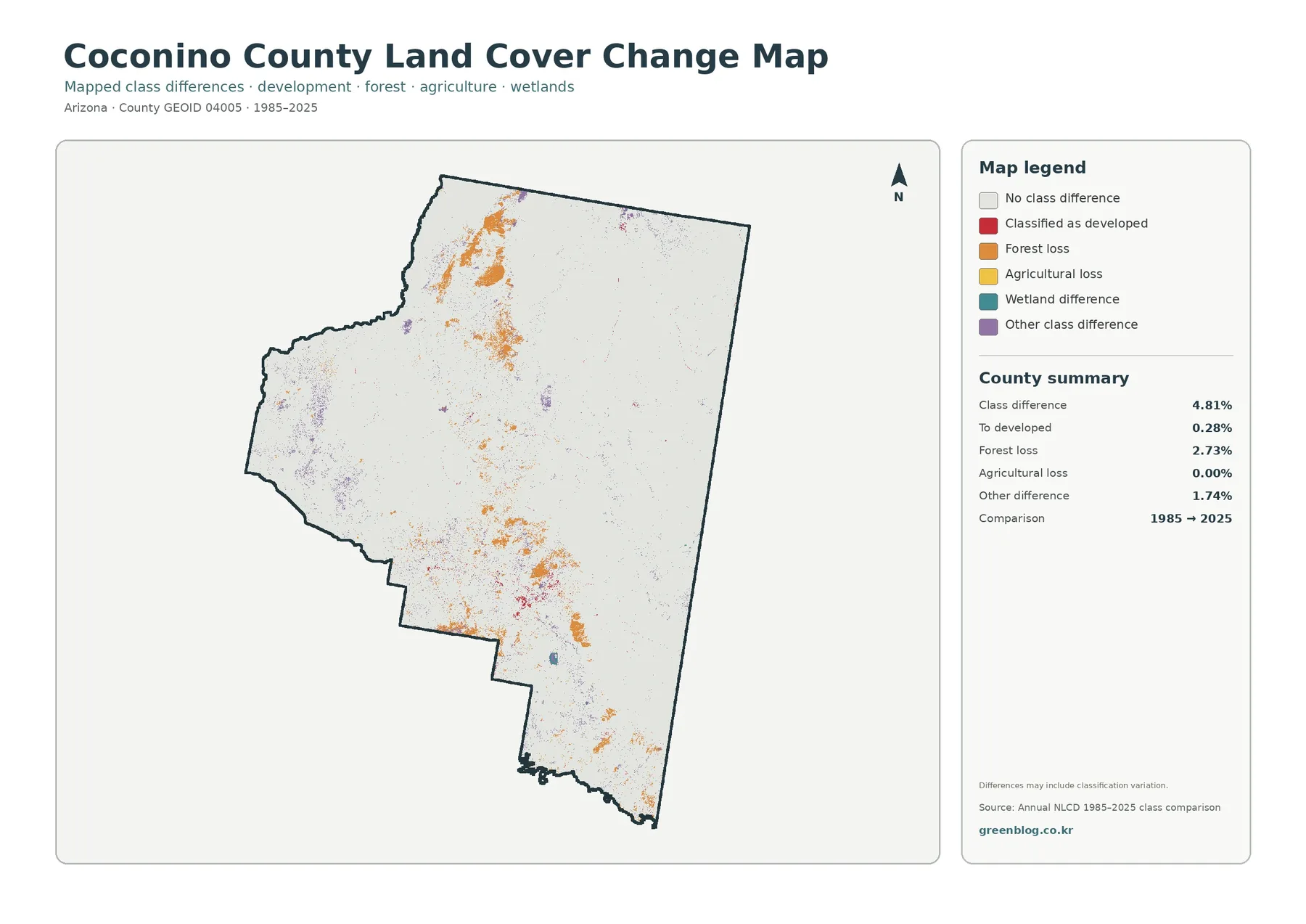
The change map separates several ideas that can easily be confused. Its 4.81% total class difference is the share of cells assigned to different land-cover classes in the 1985 and 2025 comparison. Only 0.28% is specifically labeled as transition to developed. Forest loss is listed separately at 2.73%, agricultural loss at 0.00%, and other class difference at 1.74%. The total therefore describes classification change, not a single development rate.

Orange forest-loss cells are the most noticeable change marks in parts of the north-central and southern forest zones. Red developed-transition marks are much more localized and tend to appear near existing built areas. Other class differences are scattered in multiple parts of the county. The geographic separation of these colors is useful because it shows that one process cannot explain every changed cell.

The map does not identify why a forest cell changed class. Fire, vegetation recovery, timber activity, drought, management, classification uncertainty, or another cause would need supporting evidence from other records. The safest use is to treat the map as a screening tool: locate areas that changed between the two mapped years, then consult event records, imagery, or resource-management sources for the explanation.

National parks and forests add geographic context without becoming land-cover boundaries

Coconino County’s official Helpful Links page points readers to Grand Canyon National Park, Coconino National Forest, Kaibab National Forest, and several national monuments. Those names help explain why county-scale discussions often involve very large natural landscapes. The U.S. Forest Service page for Coconino National Forest also provides a separate management context for the Flagstaff region and surrounding forested country.

These official management areas should not be traced directly from the land-cover colors. A national forest can contain shrubland, grassland, water, barren ground, and developed facilities, while forest-classified cells can occur outside a national forest. The land-cover maps describe surface condition. Park, forest, tribal, state, county, and private boundaries describe jurisdiction or ownership. Combining the two is useful only when each source keeps its own meaning.

Choose the map that matches the question instead of reading all four the same way

• Overall pattern: use the general map to compare the 71.51% shrubland majority with the major forest zones.
• Forest emphasis: use the forest-and-farmland view when the location of forest matters more than the full class legend.
• Settlement concentration: use the impervious map to show why a 0.20% countywide mean can still contain a clearly visible Flagstaff cluster.
• Time comparison: use the change map to locate 1985–2025 class differences while keeping total change, forest loss, and developed transition separate.

A classroom sequence can begin with the general map, move to the simplified forest view, then use imperviousness to discuss settlement concentration, and finish with the change map. For a presentation, fewer maps may be better. One large map with a readable legend usually communicates more than four tiny panels, so choose the view that answers the main question and use another only when a comparison adds something new.

All four maps have scale and date limitations. A roughly 30-meter cell can contain mixed surfaces, and the 2025 classification cannot show changes that happened later. Boundary pixels and small patches can also shift classification between years without representing a simple on-the-ground conversion. Current planning, engineering, legal, or site-specific decisions should use newer and more detailed sources.

Download the four Coconino County land-cover JPG maps

Frequently Asked Questions

Related Maps

• Apache County Arizona Land Cover Map
• Cochise County Arizona Land Cover Map
• From Mohave to Cochise: Reading an Arizona State Map

Sources and reference links

• MRLC Annual NLCD Data — land-cover and impervious-surface data access
• USGS Annual NLCD Land Cover Classification — class definitions and methodology context
• U.S. Census Bureau TIGER/Line Shapefiles — county boundary reference
• Coconino County Helpful Links — official links to Grand Canyon National Park, national forests, and national monuments
• U.S. Forest Service: Coconino National Forest — official forest information