San Luis Obispo County California Land Cover Map: Grassland Dominates, but Agriculture Requires a Second Look

San Luis Obispo County is dominated by open vegetation in the 2025 land-cover classification rather than by one large urban or agricultural surface. Grassland accounts for 46.13% of the county and shrubland another 32.66%, while forest forms a substantial western and interior contrast at 11.07%. Developed cover is much smaller at 4.57%, appearing in separate built clusters instead of spreading across the county as one continuous footprint.

This page includes four views of the same county: current land cover, forest and farmland, fractional impervious surface with developed land, and mapped class differences between 1985 and 2025. The four original JPG files are available together in one download below. Using the set side by side is especially helpful for separating rangeland-like open cover from mapped agriculture, comparing forested western areas with the drier interior, and seeing where hard surfaces are concentrated inside the county’s developed areas.

A broad open-land mosaic defines the 2025 county map

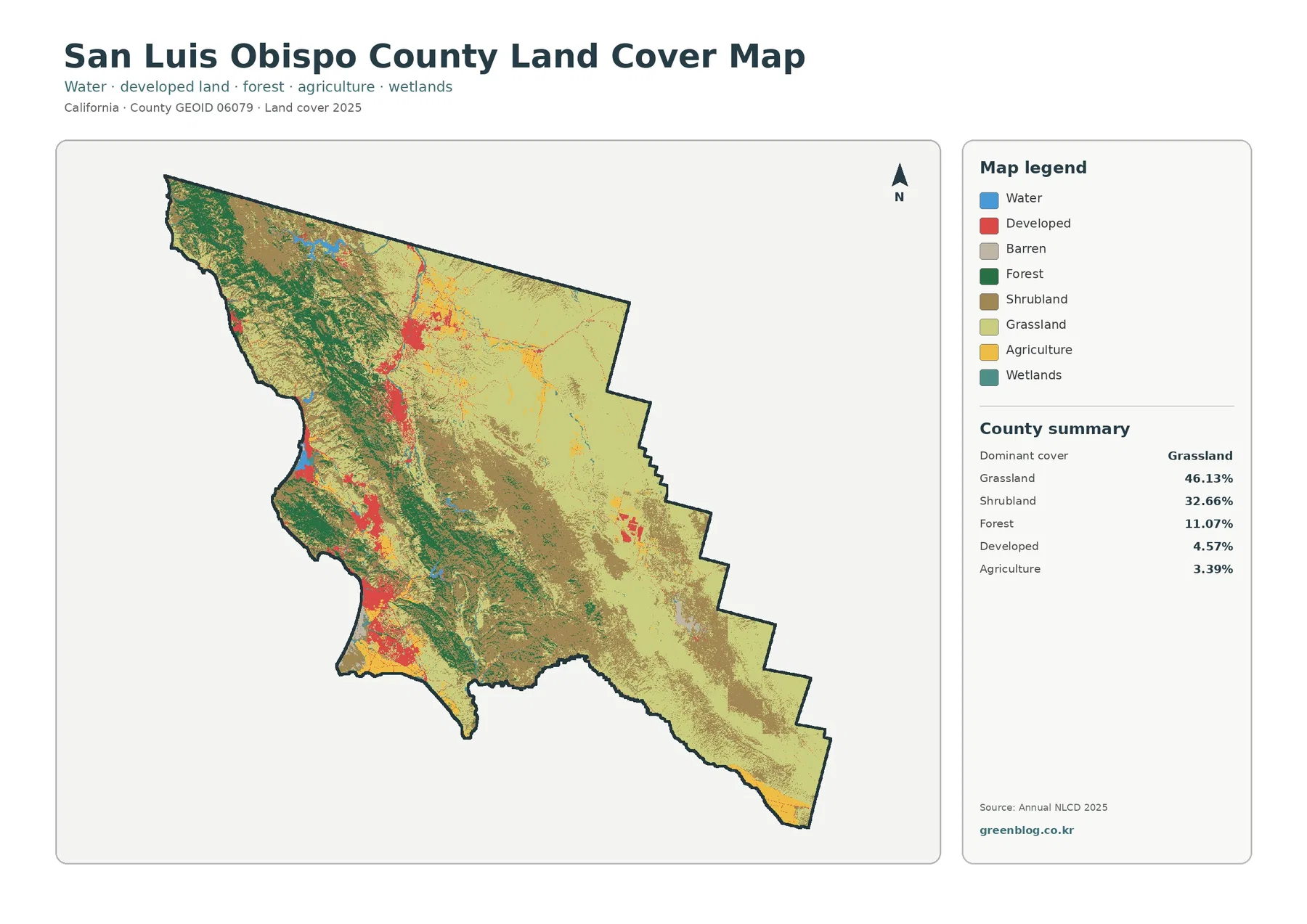
The first impression is the amount of pale grassland and brown shrubland across the interior and eastern portions of the county. Together those two classes account for most of the mapped surface. They do not form a perfectly clean division. Large patches blend into one another, while green forest, yellow agriculture, and red developed cover interrupt the open landscape in narrower bands and isolated clusters. That mixed pattern is more informative than treating the county as simply coastal, agricultural, or urban.

Forest becomes much more noticeable toward the west and northwest, with additional green bands extending through parts of the interior. The eastern and southeastern reaches contain far less continuous forest and are instead dominated by grass and shrub cover. This west-to-interior contrast can be read directly from the map without assuming that every green patch represents the same forest type or management condition. The layer classifies surface cover, not tree species, ownership, or whether a site is public or private land.

The county summary lists forest at 11.07%, developed cover at 4.57%, and agriculture at 3.39%. Water and wetlands are small enough that they are easier to study in the simplified forest-and-farmland view later on. The key point is that none of these smaller classes is evenly distributed. Forest gathers in recognizable western and interior zones, development appears as separated concentrations, and mapped agriculture occurs in several limited valleys and flatter areas rather than as one uninterrupted farming plain.

Because the dominant classes are grassland and shrubland, the map is useful for understanding why a county with important agriculture can still look mostly “natural” in a land-cover classification. Annual NLCD records what surface is most likely to occupy each raster cell. A working grazing property, for example, can still be classified as grassland if grass is the visible surface. Land cover should therefore be kept separate from legal land use, agricultural zoning, property ownership, or the economic value of farming.

Impervious cover separates the built centers from the open interior

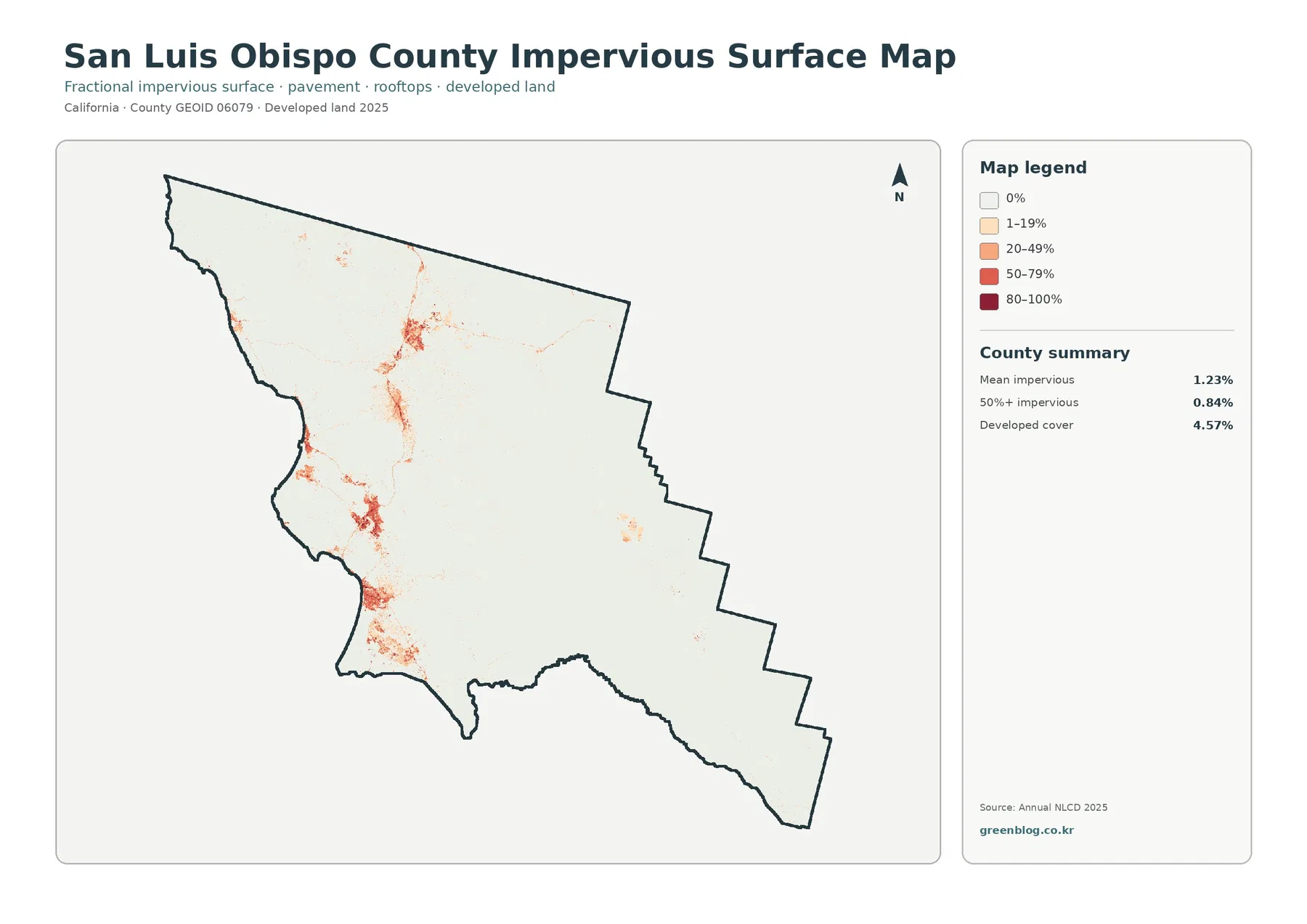
Impervious surface means hard cover such as rooftops, pavement, and parking areas where water does not readily soak into the ground. The countywide mean is only 1.23%, and 0.84% of the county is mapped at 50% impervious or greater. Those values are much lower than the 4.57% developed-cover share because developed classes can include yards, trees, lawns, vacant ground, and other permeable surfaces alongside buildings and roads.

The strongest red and orange values gather in a west-central urban concentration, with separate built clusters farther north and toward the southwestern coastal side. Thin connecting traces appear between some of those centers, but most of the county remains very pale or near zero. The pattern makes it clear that development is concentrated in several nodes rather than spread evenly through the grassland and shrubland interior. It also shows why a single developed percentage cannot describe the density of every settlement equally well.

A developed pixel and a highly impervious pixel answer different questions. The land-cover class identifies a broad developed environment, while the fractional impervious layer estimates how much of the cell is occupied by hard surface. A lower-density neighborhood can therefore appear as developed without reaching the darkest impervious category. Conversely, a compact commercial or industrial area may stand out much more strongly on the impervious map than on the general land-cover view.

Hard-surface concentration should not be treated as a flood-risk map by itself. Runoff also depends on rainfall, topography, soils, streams, drainage systems, and coastal conditions. The map is most useful for comparing the built footprint among settlements, identifying where pavement and rooftops are concentrated, and providing context before consulting dedicated stormwater, flood-hazard, or engineering data.

Forest and farmland reveal why agriculture cannot be read from one percentage

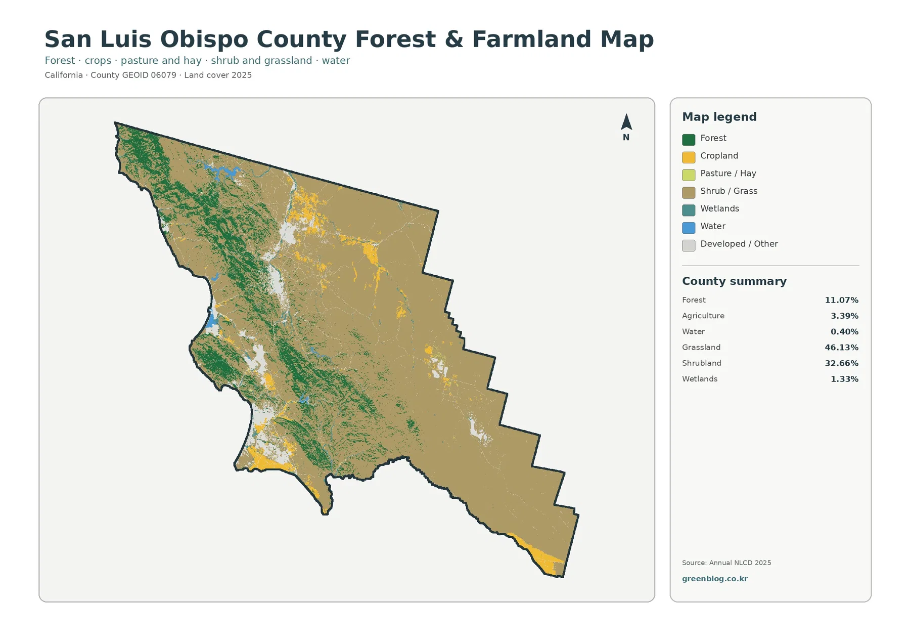
The simplified forest-and-farmland map keeps the broad open vegetation visible while making forest and agricultural cover easier to isolate. Forest remains concentrated in the western and west-central portions, with smaller green areas extending into the interior. Agricultural cover appears in several distinct pockets, including northern interior areas, central valleys, and southern or southwestern lowlands. The pattern looks more like a collection of productive valleys and flatter areas than a single countywide farm belt.

The summary for this view reports 46.13% grassland, 32.66% shrubland, 11.07% forest, 3.39% agriculture, 1.33% wetlands, and 0.40% water. Water and wetlands occupy only a small countywide share, yet blue and teal features still provide useful local reference points along the coast and at scattered inland water bodies. Their limited extent is another reminder that a small percentage can remain visually important when it is concentrated rather than evenly distributed.

San Luis Obispo County’s official Agriculture Element provides a useful local explanation for the map. It describes irrigated cropland in the Arroyo Grande and Cienega Valleys, vineyards in Edna Valley and the Paso Robles area, orchards in Nipomo Valley, dryland farming in the north county, and cattle grazing in coastal hills and interior valleys. Those examples cover several different kinds of working landscapes, not all of which would necessarily appear as the same NLCD agriculture class.

Grazing is the clearest case. A parcel can be part of an agricultural operation while its visible surface is mainly grass or shrub. In a surface-cover dataset, that location may remain grassland or shrubland rather than being assigned to a crop-oriented agriculture class. The 3.39% agriculture value should therefore not be presented as the percentage of all land used by the county’s agricultural economy. County crop reports, agricultural GIS, zoning, and land-use records answer different questions.

Local agricultural records add context without changing the land-cover numbers

The County Agricultural Resources program reports production and economic statistics, maintains agricultural mapping, and supports land-use resource protection. The annual Crop Report is designed to document what the agricultural industry produces and what that production is worth. Those records are valuable when a reader wants to understand farming as an industry, but they should not replace the 2025 land-cover percentages or be combined with them as if both datasets measure the same thing.

This distinction matters in San Luis Obispo County because the visible landscape includes vineyards, cropland, orchards, grazing land, grass-covered hills, shrublands, and forested ridges. A legal agricultural parcel can contain more than one surface type, and the 30-meter raster will assign each cell a broad classification based on the mapped surface. The resulting county summary is excellent for comparing cover patterns, but it is not a farm census and does not identify specific crops or parcel boundaries.

For a classroom or report, a useful approach is to state both ideas explicitly: the land-cover map is dominated by grassland and shrubland, while official county sources document a diverse and economically important agricultural sector. That wording avoids the false choice between the two. It also gives readers a better understanding of why rangeland and agricultural activity can overlap without forcing the map’s Grassland or Shrubland classes into a legal land-use interpretation.

The 1985–2025 layer is an endpoint comparison, not a development ledger

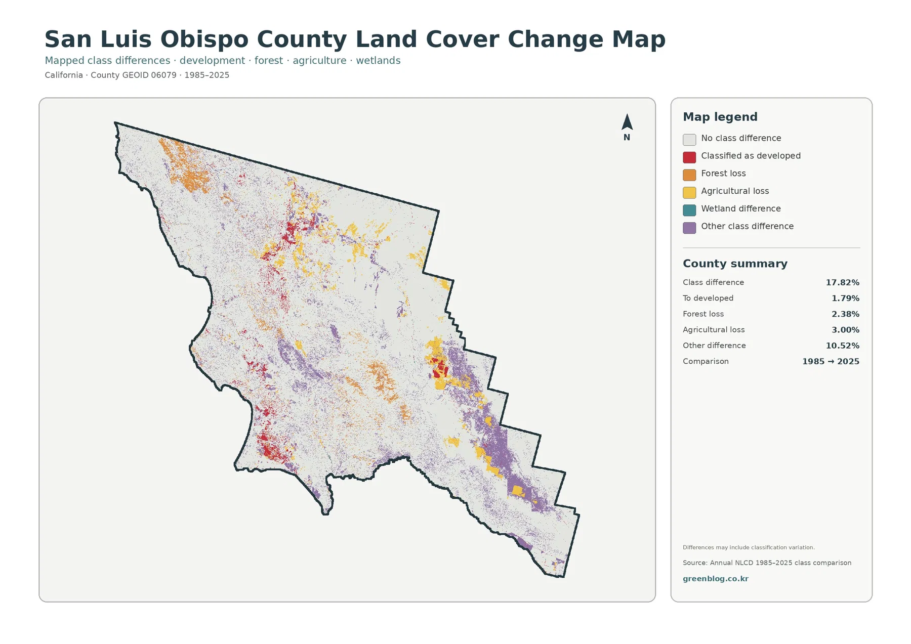
The change map reports a 17.82% class difference between the 1985 and 2025 endpoints. Within that summary, 1.79% is classified as “to developed,” 2.38% as forest loss, 3.00% as agricultural loss, and 10.52% as other class difference. Most of the county remains white, indicating no mapped class difference in this comparison, while colored patches are scattered through the north, center, east, and south.

Red developed-change cells often appear near current built concentrations and along some linear features. That spatial match is useful for locating areas worth closer study, but 1.79% should not be labeled as the exact acreage of urban expansion since 1985. The layer compares two classifications. It does not contain construction permits, subdivision dates, or a year-by-year development history.

The same caution applies to the 2.38% forest-loss and 3.00% agricultural-loss categories. They summarize how the endpoint classes differ, not timber harvest volumes, farm closures, or permanent removal of every forest or agricultural use. Vegetation condition, crop cycles, image timing, mixed pixels, and classification methods can contribute to differences. The map itself notes that classification variation may be included.

Other class difference is the largest named component at 10.52%. It combines changes that do not belong to the specifically highlighted developed, forest-loss, or agricultural-loss categories. A purple or other-change patch should not automatically be described as degradation, restoration, or development. When the reason for change matters, the stronger method is to inspect intermediate Annual NLCD years and then compare the result with aerial imagery or local records.

Choose two maps at a time for a clearer comparison

For natural-cover questions, current land cover and the forest-and-farmland map make the strongest pair. The first establishes the 46.13% grassland and 32.66% shrubland framework, while the second separates forest and agriculture more clearly. This pairing is particularly useful when explaining why working agricultural landscapes can exist inside a county that is visually dominated by grass and shrub cover.

For settlement patterns, combine current land cover with the impervious map. Developed cover identifies the broader urban footprint, while impervious intensity shows which parts of those developed areas contain the most pavement and rooftops. The two layers prevent a low-density developed area from being treated as equivalent to a compact built center simply because both belong to a developed class.

For long-term questions, place the current map next to the 1985–2025 difference map at the same size. Current built areas can be compared with “to developed” cells, forested zones with forest-loss cells, and open interior vegetation with the much larger other-difference category. Two large maps are usually easier to read in a slide or report than four small maps squeezed together, especially when the change patches and lower impervious classes need to remain legible.

Map File Information

The download ZIP contains four original JPG maps for San Luis Obispo County: current land cover, forest and farmland, impervious surface with developed land, and the 1985–2025 land-cover class comparison. Each image uses the same county boundary, which makes the set convenient for matching grassland, shrubland, forest, agricultural pockets, built clusters, and endpoint differences at the same locations.

Each source JPG in the asset manifest is 2480 by 1754 pixels. The files are identified as the original supplied images, but the manifest does not mark them as meeting an A3 high-resolution reference. If the maps will be printed large, check the legend and small change patches at the intended output size first. Resizing the image cannot create finer geographic detail than the underlying approximately 30-meter land-cover classification.

Scale, raster cells, and what the maps do not show

Annual NLCD is a raster dataset derived from Landsat imagery at 30-meter spatial resolution. In simple terms, the landscape is divided into small grid cells and each cell receives a broad mapped classification. A field edge, road, yard, patch of shrubs, and building can be close enough to share one cell. This mixed-pixel effect is why class boundaries should not be expected to follow surveyed property lines or every narrow feature exactly.

Land cover is not zoning, ownership, legal land use, or development entitlement. A grassland cell does not prove that the land is protected open space, an agriculture cell does not establish an agricultural zoning designation, and a developed cell does not identify what construction is legally permitted. Parcel and planning questions require San Luis Obispo County’s zoning, General Plan, property, and permit information rather than this surface-classification map.

The 2025 layer is also a snapshot of its mapping year. Construction, vegetation change, fire and recovery, crop rotation, water changes, or other events after the observation period may not be represented. For a current site condition, recent imagery and local records are more appropriate. For a trend, intermediate Annual NLCD years provide a stronger basis than relying only on the 1985 and 2025 endpoints.

Frequently Asked Questions

Related Maps

• Alameda County California Land Cover Map
• Alpine County California Land Cover Map
• Amador County California Land Cover Map

Sources and official references

These sources document Annual NLCD data and classification, county boundary information, and the agricultural context of San Luis Obispo County. Agricultural production, zoning, and surface cover are different subjects, so figures from one source should not be substituted for another without explaining what each dataset measures.

• MRLC Annual NLCD Data — Annual NLCD products and 1985–2025 data access
• USGS Annual NLCD Land Cover Classification — land-cover classes and classification background
• U.S. Census Bureau TIGER/Line Shapefiles — county boundary reference
• San Luis Obispo County Agricultural Resources — agricultural statistics, mapping, and resource protection
• San Luis Obispo County Crop Report — annual production and economic statistics
• San Luis Obispo County Agriculture Element — official context for valleys, vineyards, orchards, dry farming, and grazing lands