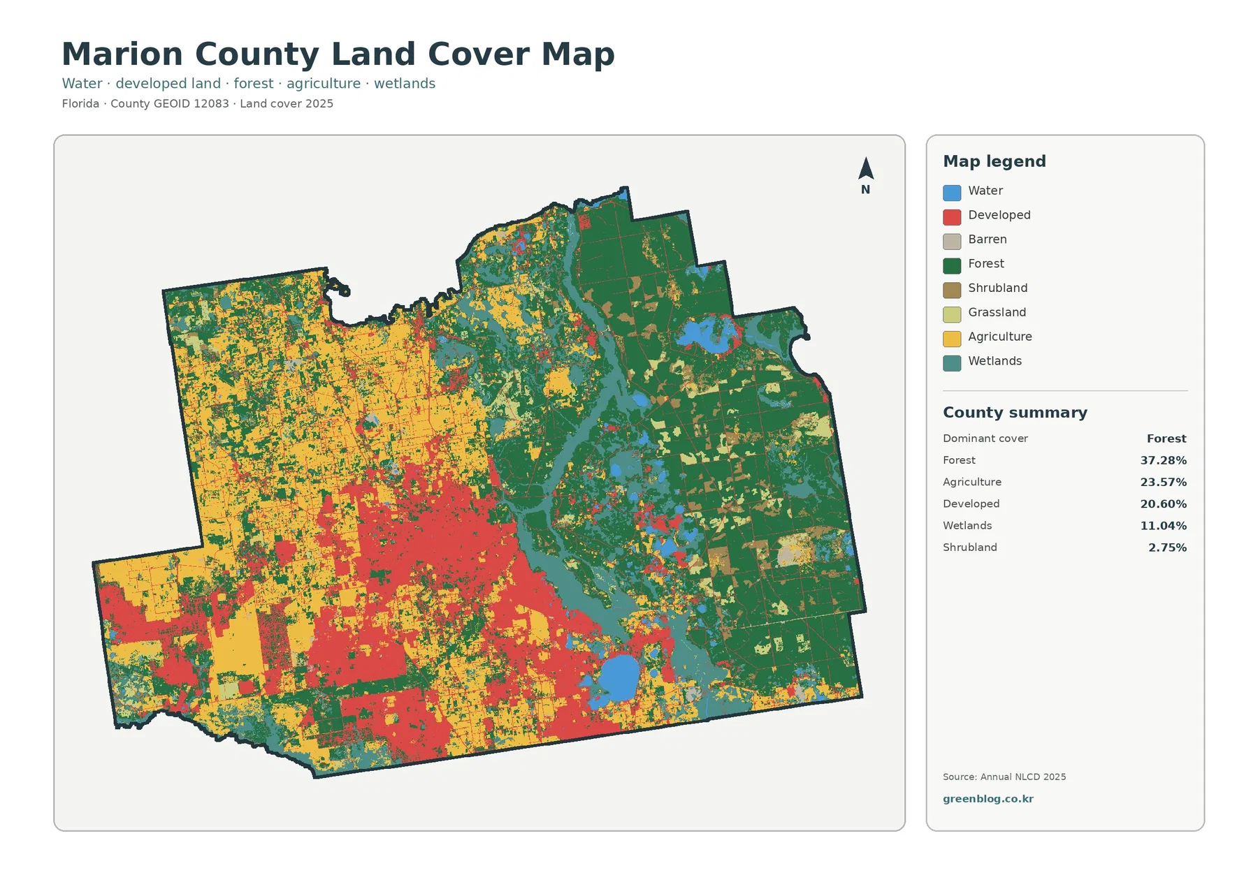
In southern Indiana, the Jefferson County Indiana Land Cover Map reveals a strong contrast: farm fields spread across the west, while broad forest cover occupies much of the east. Madison stands out as a developed concentration near the Ohio River. A large, mixed natural landscape also appears north of the city, in the direction of Big Oaks National Wildlife Refuge.
Four views let you examine that pattern from different angles: general land cover, forest versus farmland, impervious surfaces, and changes between 1985 and 2025. You can inspect the WebP previews here and get all four original JPG maps in a single ZIP. They work best as county-scale reference images rather than property surveys.
Table of Contents
A county divided between wooded hills and working fields
The 2025 county summary reports 46.57% forest and 39.24% agriculture. Developed cover accounts for 10.26%, wetlands for 2.53%, grassland for 0.68%, water for 0.33%, and shrubland for 0.27%. Forest is the leading class, but those figures alone hide an important fact: the two largest classes occupy different parts of Jefferson County.
Across the west and southwest, agricultural color forms blocks broken by smaller woods and thin natural strips. Farther east, the green areas are larger and their edges branch around narrow openings. Developed patches occur throughout the county, yet the most conspicuous built-up area is near Madison. Another concentration lies farther west along the southern side, near Hanover.
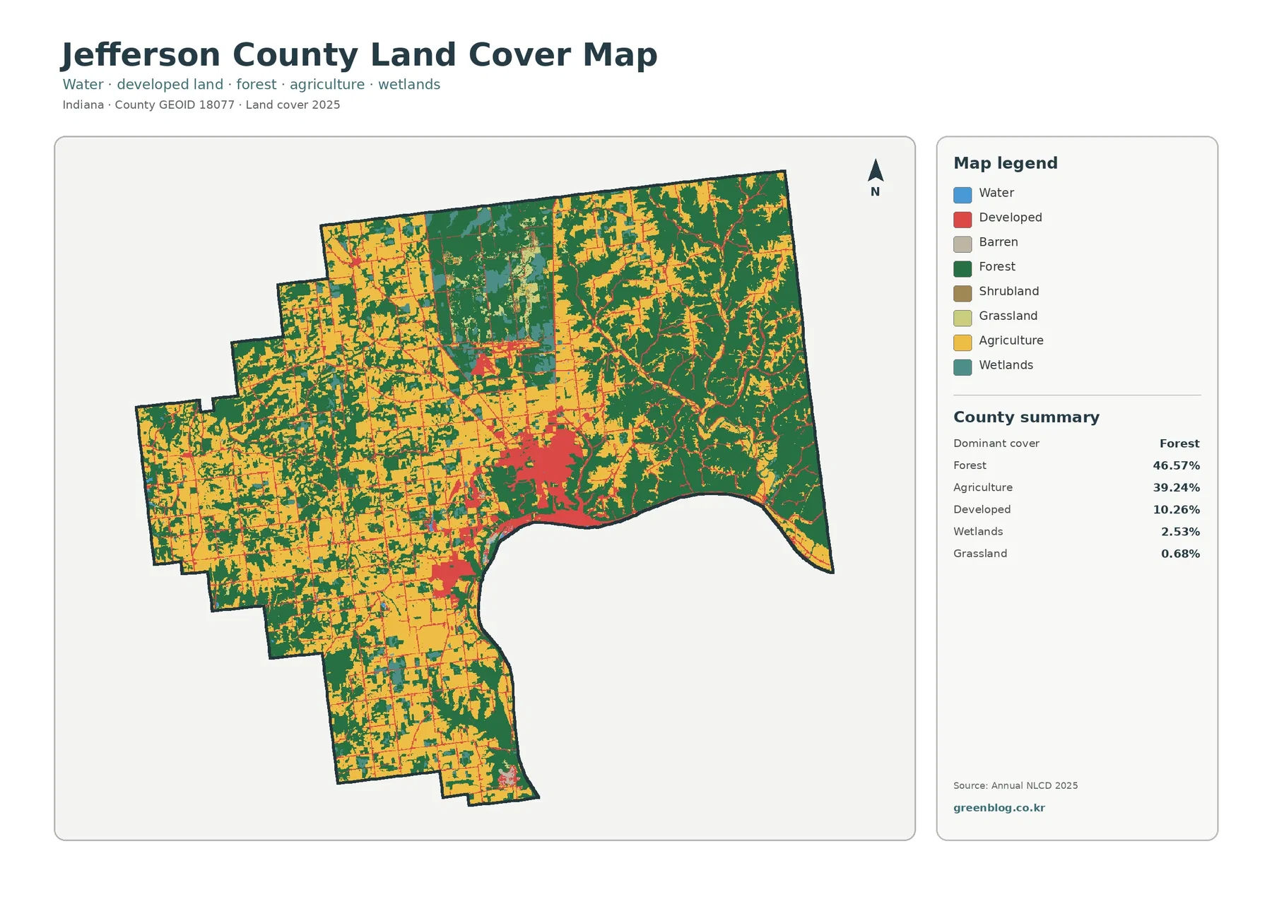
The northern middle portion deserves a closer look. It contains more than one kind of natural surface: forest appears alongside wetlands, grassy openings, and isolated developed features. Its mixture contrasts with the larger farm blocks to the west and the heavily wooded pattern to the northeast. Even within a county where two classes dominate, small wet areas and openings can reveal a different local landscape.
Land cover describes what is on the ground, not who owns a piece of land or what construction a zoning ordinance permits. An NLCD developed class can include trees and yards; an agricultural class can cross numerous properties. Madison and Hanover have distinct planning jurisdictions, but neither boundary can be drawn accurately from the color patches. For that task, consult the county planning office and official boundary data.
Why the forest–farmland border matters around Big Oaks
A second map separates forest, cropland, pasture and hay, shrub or grass, wetlands, and water. As a result, the county’s east–west contrast is easier to follow without the strong red of developed areas drawing the eye. Dark green is especially extensive toward the eastern boundary and northeast corner. Yellow and lighter agricultural tones dominate larger blocks toward the western and southwestern edges.
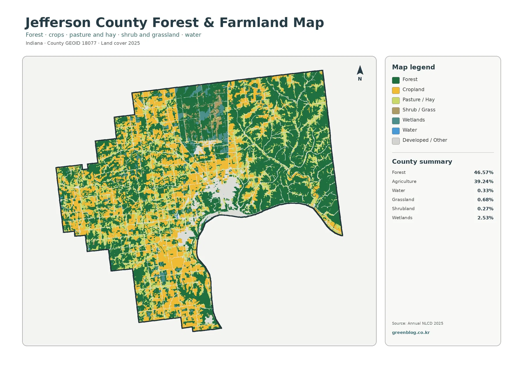
Near the center of the northern part of the map, the cover changes in a more complex pattern than ordinary fields. Big Oaks National Wildlife Refuge provides relevant geographic context. The U.S. Fish & Wildlife Service says the refuge spans Jefferson, Jennings, and Ripley counties, covers roughly 50,000 acres, and occupies part of the former Jefferson Proving Ground. Its entrance is described as about five miles north of Madison.
Those refuge facts do not mean every green or teal patch on the map belongs to Big Oaks. No refuge or property boundary is drawn in this image. Instead, read the colored cells as broad surface categories, then use official refuge maps if you need to know access, management units, or protected-land limits. The mixed forest, wetlands, and grassland in the northern area are still visible and worth comparing on their own terms.
Farm fields in western Jefferson County often have straighter edges than the branching wooded patches east of Madison. That shape difference is visible; its cause is not established by the map. Slopes, soils, landholding history, and access may all matter, but determining their influence would require additional evidence. Nor can a yellow agricultural patch tell you which crop is planted there, whether two fields have the same owner, or how much they produce.
Madison looks very different on the impervious-surface view
The third image makes human-built surfaces easier to separate from the wider developed category. Impervious cover means surfaces such as pavement and rooftops that do not readily absorb rain. On the map, a dark cluster sits in and around Madison, with thinner marks along roads and smaller settled areas. Much of the eastern woodland and the agricultural west is pale by comparison.
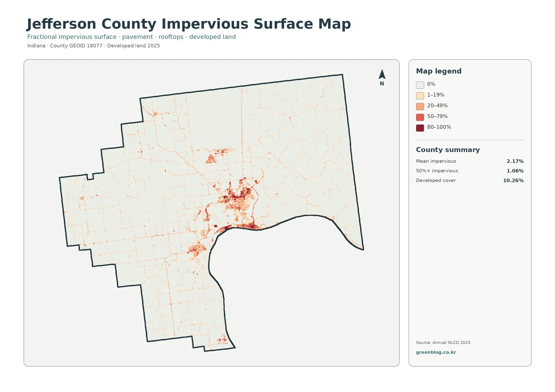
The countywide mean impervious value is 2.17%, while 1.06% of the area falls into the 50%-or-more impervious range. Neither figure conflicts with 10.26% developed land cover. A residential area may include a roof and a road together with yards, gardens, and mature trees. It can be classified as developed even when only part of its ground is covered by hard materials.
That distinction is especially useful around Madison. Compare its red developed patch in the first map with the smaller and darker hard-surface concentrations here. A second built cluster appears to the west in the Hanover direction. A long, narrow hard-surface feature is also visible north of the central built-up area. Because the map does not label it, the image alone does not establish the facility or activity associated with that shape.
A county average should never be mistaken for the condition of a particular city block. Forest and farmland occupy so much of Jefferson County that they lower the overall impervious mean. For stormwater questions, look at local topography, drains, soils, rainfall, and flood records as well. The surface map is a useful starting layer; it does not measure flooding or predict how a given street will drain.
The Ohio River boundary does not tell the whole water story
Jefferson County’s curved southern and southeastern edge follows the Ohio River corridor, but the mapped water class occupies just 0.33% of the county summary. These are different perspectives. Only cells within the county outline are counted; the broad river channel beyond it is not included. A river-basin map would answer a different question and might show a much larger water area.
Wetland cover is notably higher at 2.53%. Look for teal patches in the north-central natural landscape and thinner, broken shapes among wooded or farmed areas. Their distribution is not uniform: some cells form short corridors while others interrupt larger blocks of forest or agriculture. Small wetlands matter when comparing habitat connections and landscape variety, even if they occupy much less area than forests and fields.
Clifty Falls State Park is another important local reference near Madison. Indiana DNR describes the park’s canyon and waterfall landscape close to the Ohio River. The land-cover image shows substantial woodland near Madison and across the eastern county, but it does not mark the park’s outline. You therefore should not assign any particular green patch to the park without consulting the DNR boundary information.
A wetland class is also not a legal wetlands delineation. Water, vegetation, and nearby land can share the same grid cell, so a narrow creek or pond may not appear as a separate blue feature at this scale. These distinctions matter for environmental education. They matter even more for permit decisions, where an official delineation and site-specific evidence are essential.
What changed between 1985 and 2025—and what remains uncertain
The final image compares classifications at two endpoints, 1985 and 2025. Its headline result is a 13.20% total class difference. The summary also identifies 1.85% classified as developed, 2.05% forest loss, 0.80% agricultural loss, and 8.42% other difference; the legend has a separate wetland-difference color. These are categories of mapped comparison, not a measure of construction growth or a complete net balance for each land-cover type.
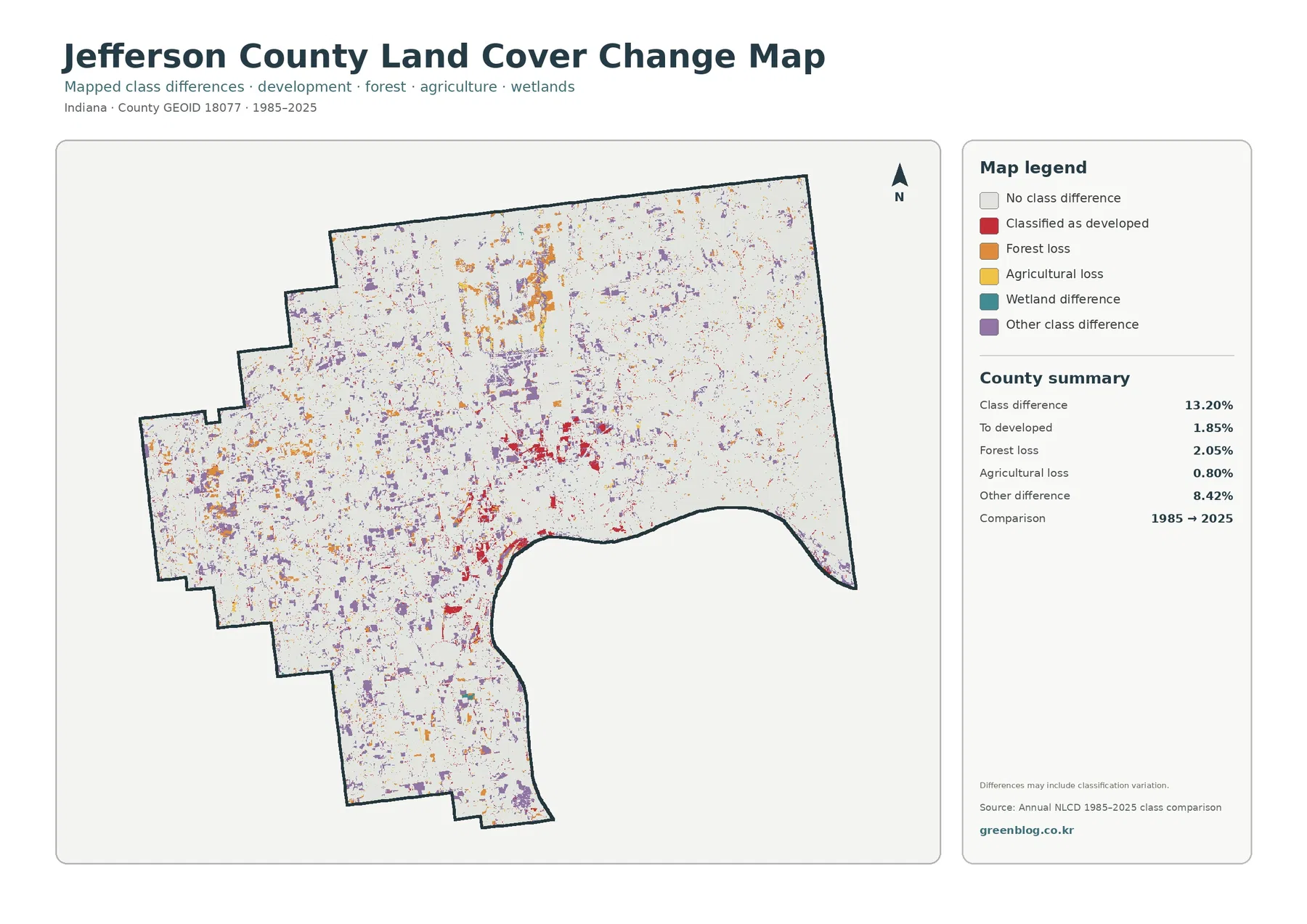
The red change-to-developed patches cluster most clearly around Madison, with smaller groups near other settled areas and routes. Orange forest-loss patches appear across more dispersed locations, while purple other-difference marks scatter through large portions of the west and north. A very light background means the representative land-cover class did not differ between the two dates.
One colored cell does not reveal exactly when a transition happened. Nor does it establish whether new construction, vegetation management, water conditions, or a classification change explains the difference. Mixed cells near woodland edges and wet ground are especially difficult to interpret. A note on the change panel warns that some differences may reflect classification variation rather than a straightforward physical conversion.
Forest-loss cells amounting to 2.05% should not be described as a 2.05% net reduction in the county’s forest cover. That figure is one reported transition class and does not subtract every possible gain elsewhere. The 0.80% agricultural-loss figure carries a similar limitation. Use the map to locate potential changes, then review intermediate annual imagery, historical photos, or local records before drawing conclusions about causes or timing.
A practical route through the four Jefferson County maps
For a quick county overview, begin with the general cover map and identify three anchors: the Madison developed cluster, the western agricultural blocks, and the eastern wooded area. The forest-and-farmland image is a useful second step because it lets you compare the shapes and extent of the two dominant cover groups without competing colors.
Next, examine the hard-surface layer at those same locations. Madison’s streets and developed core become more distinct, while forest and farmland contain mostly faint marks. Compare that pattern with the change image only after you have the current geography in mind. A red cell in the change map tells you a classification differs at the historical endpoints; it does not automatically mean a new neighborhood appeared recently.
For a classroom or slide presentation, place the four JPG maps at the same orientation and similar size. One useful exercise traces the northern natural-cover patch across the overview and the forest map before checking it for orange, purple, or teal change categories. Another follows the Ohio River-side developed concentrations through the impervious layer. Keeping the year and legend alongside each image prevents confusion.
Scale, sources, and sensible limits
These maps are county-scale interpretations of Annual NLCD land-cover products for 2025, with the change panel comparing the 1985 and 2025 endpoints. The mapped surface is generalized into raster cells; the 30-meter scale can blend a narrow stream, a road, small buildings, and adjacent vegetation into one representative category. Fine parcel boundaries cannot be recovered from those cells.
Colors also mean different things across the four panels. Red in the overview is developed cover, deeper tones in the impervious view indicate a larger share of hard surface, and red in the historical comparison refers to a change-to-developed category. Read each legend separately. The four maps are complementary precisely because none of them supplies the same measurement as the others.
For conservation, zoning, or construction decisions, supplement the images with authoritative property lines, permits, current aerial photography, on-site checks, and applicable agency records. The comparison does not capture changes after 2025. What these views do provide is a clear geographic framework for asking better questions about Jefferson County’s forest, farms, town centers, and natural areas.
Frequently Asked Questions
Is the large green area north of Madison all part of Big Oaks?
No. Big Oaks is relevant local context, but these images show land-cover classes rather than refuge boundaries. Confirm land ownership and access using official refuge maps.
Why does developed cover exceed impervious cover by so much?
The developed class can include lawns, trees and other permeable ground. Impervious data focuses on roofs, pavement and similar hard surfaces, so its countywide average answers a different question.
Does 13.20% class difference mean Jefferson County became 13.20% more urban?
No. The total includes several land-cover transitions and possible classification variation. Only 1.85% appears in the map’s change-to-developed category, which itself is not a dated construction statistic. Map File Information This ZIP holds four original JPG maps of Jefferson County: 2025 land cover, forest and farmland, impervious/developed surfaces, and the 1985–2025 class comparison.
Map File Information
Download one ZIP archive containing the four original land-cover map JPG files.
- Included Files: Four original land-cover map JPG files
- File Type: ZIP archive containing four JPG files
- Intended Use: Map comparison, learning, and print reference
Related Maps
- Adams County Indiana Land Cover Map
- Allen County Indiana Land Cover Map
- Bartholomew County Indiana Land Cover Map
Sources and references
- MRLC Annual NLCD Data — annual land-cover data and documentation
- USGS Annual NLCD Land Cover Classification — definitions for mapped surface classes
- U.S. Fish & Wildlife Service – Big Oaks — refuge geography and habitat context
- Indiana DNR – Clifty Falls State Park — landscape information near Madison
- Jefferson County Planning & Zoning — official planning information separate from the land-cover classes
Green Map creates custom-edited map images using open geographic data sources such as geoBoundaries, Natural Earth, OpenStreetMap, and government open data. These maps are edited visual materials, not raw data files, and are provided for education, documents, presentations, and graphic reference.