Glades County has a 2025 land-cover pattern unlike a heavily urban Florida county. Wetlands account for 37.16% of the mapped area and agriculture is almost equal at 36.82%. Lake Okeechobee forms a large water presence along the eastern side, while broad agricultural blocks are more prominent to the north, west, and south. The four maps on this page separate those patterns into general land cover, forest and farmland, impervious surface, and 1985–2025 class differences.
The WebP images are designed for quick viewing in the article, and the four original JPG maps are available together in one download below. Land cover describes what the ground surface was classified as from remotely sensed data; it is not a zoning map, ownership map, or parcel survey. These maps are useful for county-scale comparison, but legal land use and site-level decisions require more detailed local records.
Table of Contents
Wetlands and agriculture divide most of the county between them
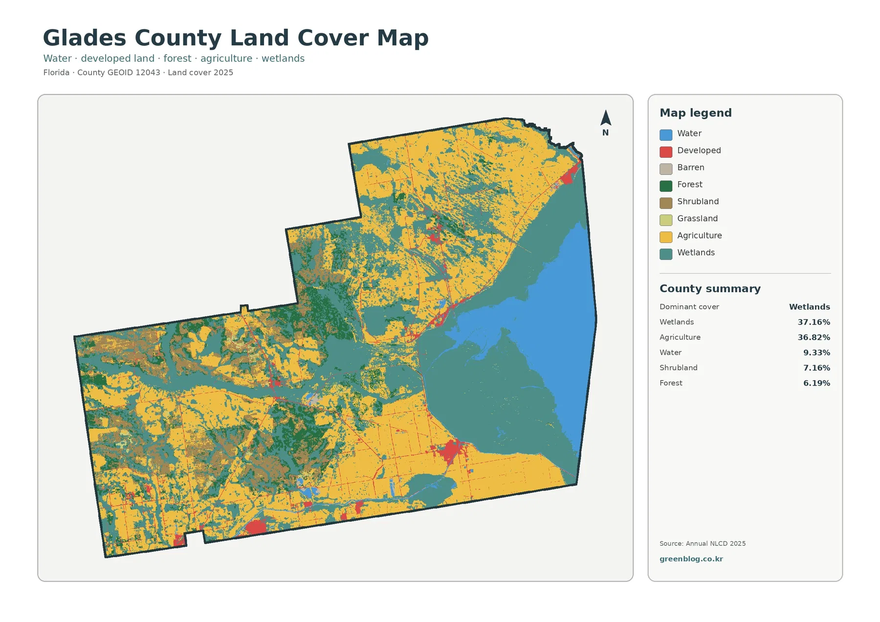
The strongest visual contrast comes from teal wetlands and yellow agricultural land. Wetlands cover 37.16% and agriculture covers 36.82%, a difference of only 0.34 percentage points. Neither category overwhelms the county by itself. Together, however, they occupy roughly three quarters of the mapped area, so any useful description of Glades County has to consider both the working landscape and the water-influenced landscape.
Water makes up 9.33% of the county summary and is concentrated most clearly on the eastern side where Lake Okeechobee enters the county map. A broad wetland belt lies immediately west of much of that open water. The South Florida Water Management District describes Lake Okeechobee as a central water body in the Greater Everglades watershed, which provides useful geographic context for the large water-and-wetland zone visible here. The land-cover image itself does not define the lake’s management boundaries or changing shoreline stages.
Shrubland accounts for 7.16% and forest for 6.19%. Both appear in smaller patches across the western and central parts of the county, often between agricultural areas and wetlands. Grassland is only 0.48% in the summary, and barren land is also represented in the legend as a minor class. Those small categories are easy to miss at page scale, which is one reason the JPG files are more useful when a reader wants to enlarge the legend and inspect individual patches.
Developed cover is 2.69%. Red areas are not spread evenly across the map; they appear as small clusters and thin connections within a much larger matrix of agriculture, wetlands, and other open land. Because this map does not label town limits or road names, those red patches should not be treated as exact municipal boundaries. Their main value is showing how limited the developed footprint is relative to the county as a whole.
The forest-and-farmland view makes the working-land pattern easier to follow
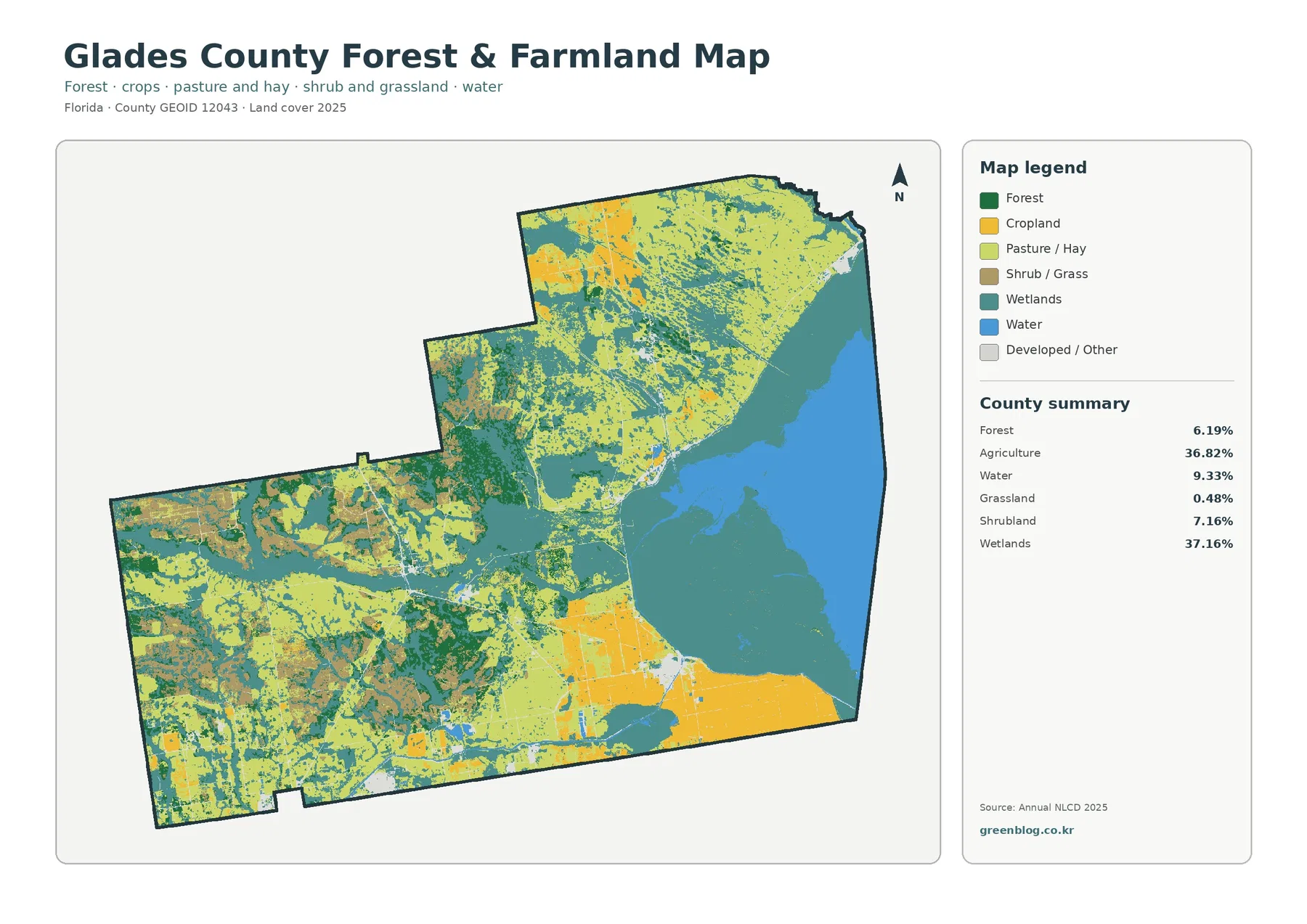
Agricultural land becomes especially clear in this version because the map gives working land and natural cover more visual emphasis. Large yellow blocks extend across the north and south, while the western side contains a more mixed pattern of agriculture, shrub or grass cover, forest, and wetlands. Moving toward the center and east, wetlands and open water become more prominent. The county therefore does not have a simple farm-versus-natural-land split; several cover types meet along broad transition areas.
The 36.82% agricultural share is consistent with the importance of agriculture in local extension work. UF/IFAS Extension Glades County lists agriculture and natural resources among its program areas and operates in partnership with Glades County Government and USDA. That local context supports describing agriculture as an important county activity, but the yellow map class should not be read as a crop inventory. A land-cover raster does not identify individual crops, ranch ownership, or parcel boundaries.
Wetlands remain nearly as extensive as agriculture in this focused map. Along the eastern side they occupy a large continuous-looking area beside Lake Okeechobee, while farther west they break into narrower and more irregular patches. The map is useful for seeing where agriculture and wetlands lie close together, but proximity is not evidence that one caused the other. Drainage, soil, water management, land history, and seasonal conditions would need separate evidence.
Forest is a smaller countywide category at 6.19%, yet its darker green patches help distinguish the western and central mosaic from the more open agricultural blocks. Shrubland at 7.16% is slightly larger and often appears around the same broad part of the county. Those two classes should still be kept separate: the map does not provide species, canopy height, stand age, or management condition, so it cannot support detailed ecological conclusions from color alone.
A 0.67% mean impervious value reveals how sparse hard surfaces are
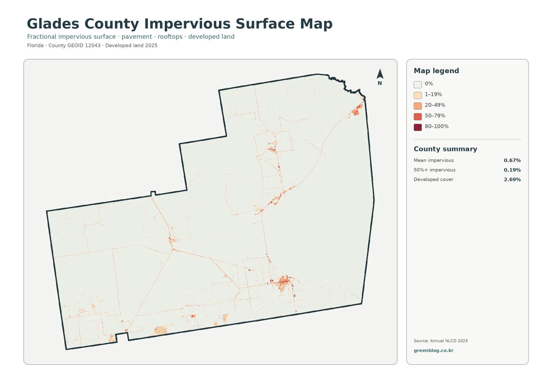
Impervious surface means hard cover such as pavement, parking areas, and rooftops where rainfall does not easily soak into the ground. The countywide mean is 0.67%, and only 0.19% of the mapped area has imperviousness of 50% or more. Developed land is larger at 2.69% because a developed class can include lawns, bare soil, trees, yards, and other surfaces that still allow some infiltration.
Most of this map is very pale. Darker values are limited to a few compact clusters, with one particularly visible concentration in the southern part of the county and smaller concentrations toward the center and northeastern edge. Thin road-like traces connect some of these places. The pattern is much different from a county where dense development forms a broad continuous field, and it explains why the mean impervious value remains below one percent.
UF/IFAS Extension Glades County is located in Moore Haven, giving readers one verified local reference point for the county’s community geography. The impervious map itself does not label Moore Haven, roads, or census places, so individual clusters should not be assigned to a named settlement without a separate base map. Pairing this image with an official road or municipal map is the better way to identify specific locations.
Low impervious cover should not be confused with low flood or drainage risk. Glades County includes large wetlands, agricultural areas, and a major lake edge, so water movement depends on rainfall, water levels, canals, levees, soils, topography, and drainage infrastructure as well as pavement. A parcel-level flood question requires current flood maps and site-specific data rather than a countywide impervious image.
Lake Okeechobee explains why open water and wetlands must be read separately
Lake Okeechobee is the most obvious named geographic feature tied to the eastern side of the map. The South Florida Water Management District describes it as a roughly 730-square-mile shallow lake at the center of a much larger watershed, while the Florida Fish and Wildlife Conservation Commission notes that it borders Glades County and several neighboring counties. That context helps explain why Glades County has a substantial 9.33% water class alongside an even larger wetland class.
Blue open water and teal wetlands represent different surface conditions. Open water accounts for 9.33%, while wetlands account for 37.16%. The two categories touch across much of the eastern part of the county, but they should never be combined automatically or treated as the same thing. Wetland classes can contain vegetation and seasonally or persistently wet ground that is not mapped as open lake water.
The wetland boundary has many irregular edges and narrow extensions. At the scale of a 30-meter raster classification, small channels, emergent vegetation, exposed ground, and adjacent land can fall within the same or neighboring cells. The line between colors is therefore a generalized representation rather than a surveyed wetland boundary. Regulatory or permitting work needs agency-specific wetland and hydrologic information.
The same caution applies where agricultural blocks meet wetland colors. Their close placement is a visible fact, but the map does not reveal farm drainage systems, irrigation sources, water-control operations, or nutrient movement. Those questions belong to hydrology, agricultural management, and water-quality datasets. The land-cover map is best used to locate broad areas where a more detailed investigation may be worthwhile.
The 1985–2025 comparison marks class differences, not a single change rate
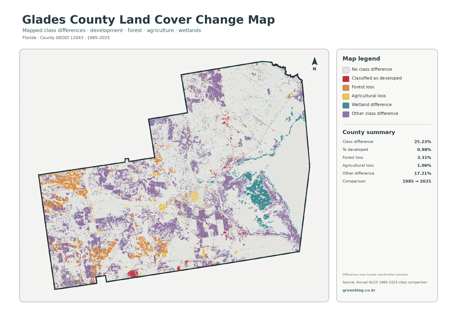
The change map reports a total class difference of 25.23% between 1985 and 2025. Within that comparison, 0.98% is classified as a transition to developed land, 3.31% as forest loss, 1.06% as agricultural loss, 2.67% as wetland difference, and 17.21% as other class difference. Because the “other” category is by far the largest component, the total cannot be explained simply as urban growth or the loss of one land-cover class.
Differences are scattered across the county rather than confined to one corridor. Orange forest-loss patches and purple other-class differences are especially noticeable in the west and southwest. Teal wetland differences occur around parts of the central and eastern wetland zone, while red developed transitions appear in comparatively small clusters and thin lines. The spatial mix is more informative than the total percentage alone.
A note on the map states that differences may include classification variation. That warning matters. Two dates can be assigned different classes because of actual land change, but imagery, vegetation condition, seasonal moisture, or classification methods can also contribute. The 3.31% forest-loss figure and 1.06% agricultural-loss figure should therefore not be presented automatically as permanent net losses.
Anyone investigating a specific change area should compare intermediate Annual NLCD years, aerial imagery, agricultural records, and water-management information. That is particularly important in a county where agriculture and wetlands each cover more than one third of the landscape. Seasonal water and vegetation conditions may affect how some cells are classified, and a two-endpoint comparison cannot describe every transition that happened during the forty-year period.
Using all four maps prevents misleading countywide conclusions
The general land-cover map is the best starting point when the question is simply, “What covers Glades County in 2025?” It puts the 37.16% wetland share and 36.82% agricultural share in one view and shows the strong east-west contrast between Lake Okeechobee-related water and the county’s broad working lands. For a presentation or county overview, it is the most complete single image.
The forest-and-farmland map is better when agriculture needs to be compared directly with forest, shrub or grass cover, and wetlands. It removes some visual competition from the developed classes and makes the mixed western landscape easier to follow. That makes it useful for environmental education, agriculture discussions, or county comparisons where the relationship between working land and natural cover matters more than settlement density.
The impervious map answers a narrower question: where are rooftops, pavement, and other hard surfaces concentrated? Its 0.67% mean gives a very different impression from the 2.69% developed-cover figure, and that difference is meaningful rather than contradictory. Developed land can contain substantial permeable ground. Showing both numbers helps avoid describing every developed cell as fully paved.
The change map should come last because it depends on understanding the present-day pattern first. A red or orange change patch means more when the reader can return to the 2025 land-cover map and see what covers the area now. Using the maps together also prevents the 25.23% total class difference from being mistaken for a simple countywide land-loss or development rate.
Resolution, classification, and date limits matter when printing or comparing maps
Each downloadable JPG is 2480×1754 pixels. That size works well for documents, slide decks, and many screen-based uses, but it is below a full A3 image at 300 dpi. A large poster may still be usable depending on viewing distance, yet readers should test the intended print size before relying on very small legend text or narrow map details.
Annual NLCD data are raster based, meaning the landscape is divided into grid cells and each cell receives a class. Narrow roads, small drainage features, field edges, and tree lines can be mixed within a cell. Enlarging the JPG makes the pixels bigger; it does not create parcel-level detail that was not present in the original classification.
The maps represent 2025 land cover and a 1985–2025 endpoint comparison. Construction, agricultural conversion, restoration, vegetation change, or flooding after the observation year may not be represented. When current conditions matter, combine these maps with recent aerial imagery and present-day local records.
Comparisons with another county are strongest when both maps use the same year and the same classification definitions. Mixing a 2025 Glades County map with an older land-cover product from somewhere else can blend real geographic differences with differences in time or methodology. Keeping the source year consistent makes percentages and visible patterns more meaningful.
Download the four Glades County JPG map files
The ZIP contains one JPG for each of the four views: 2025 general land cover, forest and farmland, impervious surface and developed land, and the 1985–2025 land-cover class comparison. Use the WebP images for quick reading on the page and the JPG files when you need to enlarge the legend, place a map in a document, or compare it beside another county.
Choose the map according to the question. The general map is best for an overall county profile, the forest-and-farmland version emphasizes the 36.82% agricultural and 37.16% wetland balance, the impervious map isolates the sparse hard-surface footprint, and the change map locates areas where the two endpoint classifications differ.
Frequently Asked Questions
What is the largest 2025 land-cover class in Glades County?
Wetlands are the largest class at 37.16%, with agriculture close behind at 36.82%. Water accounts for 9.33%, shrubland 7.16%, and forest 6.19%. The eastern Lake Okeechobee side is dominated by water and wetlands, while broad agricultural areas are more prominent farther north, west, and south.
Why is developed cover 2.69% when mean impervious surface is only 0.67%?
A developed land-cover class can contain lawns, trees, bare soil, drainage areas, and other permeable surfaces in addition to pavement and buildings. Impervious surface measures the harder fraction more directly. Only 0.19% of the county has imperviousness of 50% or more, which matches the small, concentrated dark patches visible on the map.
Does the teal area next to Lake Okeechobee represent open lake water?
No. Blue represents open water and teal represents wetlands. Water is 9.33% of the county summary, while wetlands cover 37.16%. The two classes lie next to each other across much of the eastern side, but wetlands can include vegetated or seasonally wet ground and should not be counted as open water.
Map File Information
Download the four Glades County land-cover JPG maps together in one ZIP file.
- Included Files: Use only the versions confirmed in the article and supplied images
- File Type: Use the confirmed download contents
- Intended Use: Printing, education, presentations, and map-based projects
Related Maps
- Alachua County Florida Land Cover Map
- Baker County Florida Land Cover Map
- Bay County Florida Land Cover Map
Sources and References
- MRLC Annual NLCD Data – official access point for Annual NLCD land-cover datasets.
- USGS Annual NLCD Land Cover Classification – definitions and guidance for the mapped land-cover classes.
- South Florida Water Management District – Lake Okeechobee – official lake, watershed, water-management, and ecological context.
- UF/IFAS Extension Glades County – local agriculture and natural-resources extension information.
- U.S. Census Bureau TIGER/Line Shapefiles – official county boundary source.
Green Map creates custom-edited map images using open geographic data sources such as geoBoundaries, Natural Earth, OpenStreetMap, and government open data.
These maps are edited visual materials, not raw data files, and are provided for education, documents, presentations, and graphic reference.