Custer County Colorado Land Cover Map — Westcliffe in an Open Valley Between Forested Ranges

Custer County sits in a high mountain setting where the land-cover pattern changes sharply between the Wet Mountain Valley and the ranges on either side. In the 2025 summary, forest is the largest class at 39.84%, followed by shrubland at 27.79% and grassland at 21.78%. Agriculture and wetlands occupy much smaller shares, while developed cover is concentrated around the neighboring towns of Westcliffe and Silver Cliff rather than spread broadly across the county.

This page brings together four views of the same county: current land cover, forest and farmland, impervious surface and developed land, and mapped change from 1985 to 2025. The maps can be compared on the page, and the four original JPG files are available together in one ZIP download. That makes the set useful when you need a countywide reference for a class, presentation, regional study, or visual comparison.

A broad valley separates two very different mountain edges

Custer County is in south-central Colorado. County planning material describes most of the county as mountainous, with the Sangre de Cristo Range forming the western side and the Wet Mountains occupying the northeast. Westcliffe and Silver Cliff sit close together in the Wet Mountain Valley between those higher areas. That physical setting is easy to recognize in the land-cover maps even though the maps are not topographic: forest dominates large mountain blocks, while the middle of the county contains more grassland, shrubland, agricultural cover, wetlands, and a compact developed area.

The contrast matters because the county is not simply a continuous forest. Forest accounts for 39.84%, but shrubland and grassland together make up almost half of the mapped area. The open central valley is therefore a major part of the county’s visual pattern, not a narrow break between mountain forests. Agricultural cover and wetlands add smaller but locally distinct patches within that open area, and the developed footprint is small enough that it does not dominate the county map.

Official county information also places DeWeese Reservoir at the north end of the Wet Mountain Valley. The current land-cover map contains a small water feature and surrounding wetland colors in that northern valley setting. Knowing the verified landscape names helps orient the map, but the colors should still be read as surface-cover classifications. They do not identify ownership, zoning districts, building rights, or parcel boundaries.

Reading the 2025 land-cover pattern

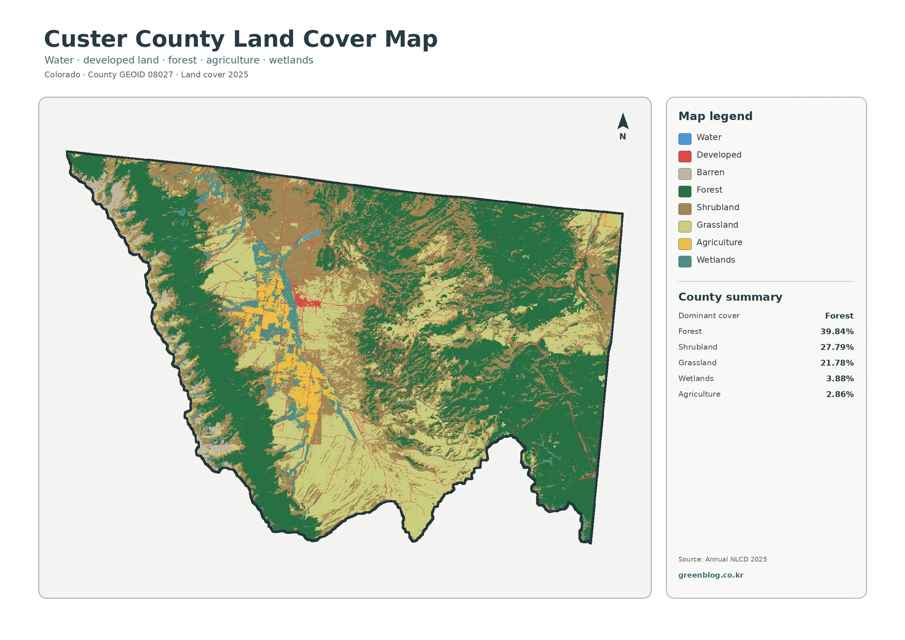
The general land-cover map is the best starting point because it keeps the full range of classes visible. Forest leads the county summary at 39.84%, shrubland accounts for 27.79%, and grassland covers 21.78%. Wetlands are 3.88%, agriculture is 2.86%, and water is 0.08%. Those smaller percentages are still important because they are not evenly scattered. They form recognizable patches and narrow areas within the central valley, so location adds information that the countywide percentages alone cannot provide.

Dark green forest covers broad sections along the western mountain side and across much of the eastern high ground. The center of the county changes to lighter grass and shrub colors, with agricultural patches appearing more often along the valley. Wetland colors form narrow and irregular features through portions of the same central area. A compact red developed patch near the middle stands out because it contrasts strongly with the surrounding natural cover, even though developed land occupies only a small share of the county.

Land-cover pixels should not be treated as surveyed property lines. Annual NLCD maps the landscape as raster cells, which are small grid squares that receive a classification based on the underlying data. A narrow stream, forest edge, road, or small group of buildings may share a cell with another cover type. At county scale, the map is strongest for comparing broad concentrations and transitions. It is not designed to answer whether one specific parcel is entirely forest, wetland, or agricultural land.

Forest wraps around an open valley of grass, shrub, and farm cover

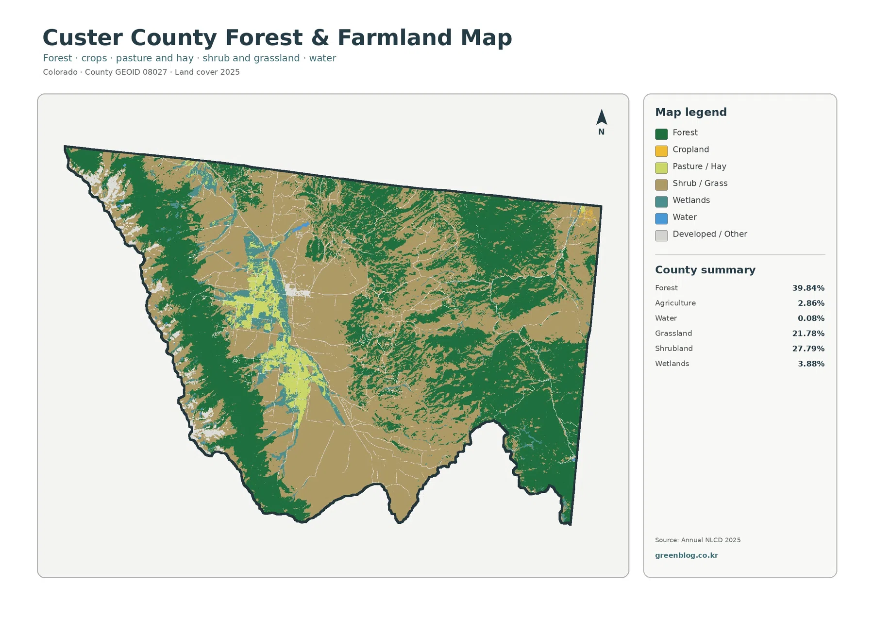
The forest and farmland view removes some of the complexity of the general map and makes the mountain-valley divide easier to follow. Forest forms large connected areas on the west and east sides. The Wet Mountain Valley in the center contains much more shrub and grass cover, along with pasture or hay and smaller cropland patches. Agriculture is only 2.86% in the county summary, yet its clustering in the valley makes it more visible than the percentage might suggest.

Wetlands cover 3.88%, slightly more than the mapped agricultural class, and they often appear as narrow features through the open valley rather than large blocks. Water is just 0.08%, so blue areas are limited. The verified location of DeWeese Reservoir at the north end of the valley provides a useful reference point for interpreting the small northern water feature. On a reduced map, these narrow classes can be easy to miss, so zooming in is helpful when the goal is to compare water and wetland cover with nearby grass or agricultural land.

The distribution should be described as an association, not a cause-and-effect story. The map shows agricultural and open-land classes concentrated in the valley and forest concentrated in the mountains. It does not by itself explain whether elevation, soil, irrigation, ownership, or another factor produced each patch. Those questions require other datasets. For this map, the reliable observation is the strong difference in surface cover between the forested ranges and the more open central valley.

It is also important not to confuse “farmland” on this thematic map with a legal land-use designation. The colors represent land-cover classes derived from remotely sensed data. They do not mark farm ownership, agricultural zoning, conservation easements, or exact field boundaries. Custer County maintains separate GIS and zoning resources for those subjects, which is why a land-cover map should be used as environmental context rather than a substitute for official parcel or planning information.

The built footprint is small and centered near the two towns

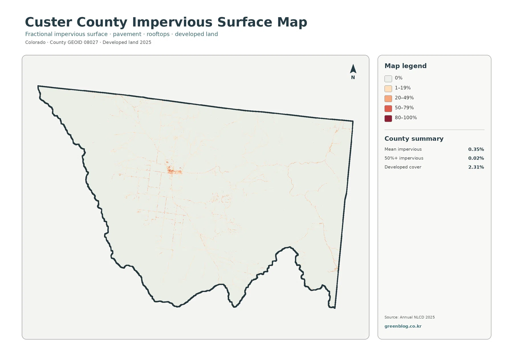
Impervious surface means ground covered by materials such as pavement and rooftops that do not readily absorb water. On this map, most of Custer County remains near the lightest end of the scale. The county summary reports a mean impervious value of 0.35%, only 0.02% of the area at 50% or greater imperviousness, and 2.31% developed cover. Those numbers fit the visual impression: intense built surfaces occupy a very small part of a largely forested and open landscape.

The strongest cluster appears in the central valley where Westcliffe and Silver Cliff are located next to one another. Thin lines and small marks extend away from that cluster, but the map does not label individual roads or buildings. A visible line should therefore be treated as a mapped impervious pattern, not proof that every part of the cell is pavement. The percentage scale refers to the share of hard surface within a cell, which is different from simply labeling the entire cell as developed land.

Comparing this map with the general land-cover view helps prevent a common visual mistake. Red developed pixels draw attention quickly on the general map because they contrast with green, tan, and yellow surroundings. The impervious map puts their scale in perspective: the great majority of the county stays pale, while the more noticeable colors are limited to the town area and scattered narrow features. This makes the map useful for explaining not just where built surfaces occur, but how small their countywide footprint is.

The map is not a permit or development-potential map. It cannot tell a property owner whether a parcel can be subdivided, where a new structure may be built, or which roads are public. Those questions belong with Custer County Planning & Zoning and official GIS records. For watershed or environmental comparisons, however, the impervious layer offers a clear complement to the forest and grassland maps because it isolates the hard-surface pattern from the rest of the landscape.

What changed between the 1985 and 2025 classifications

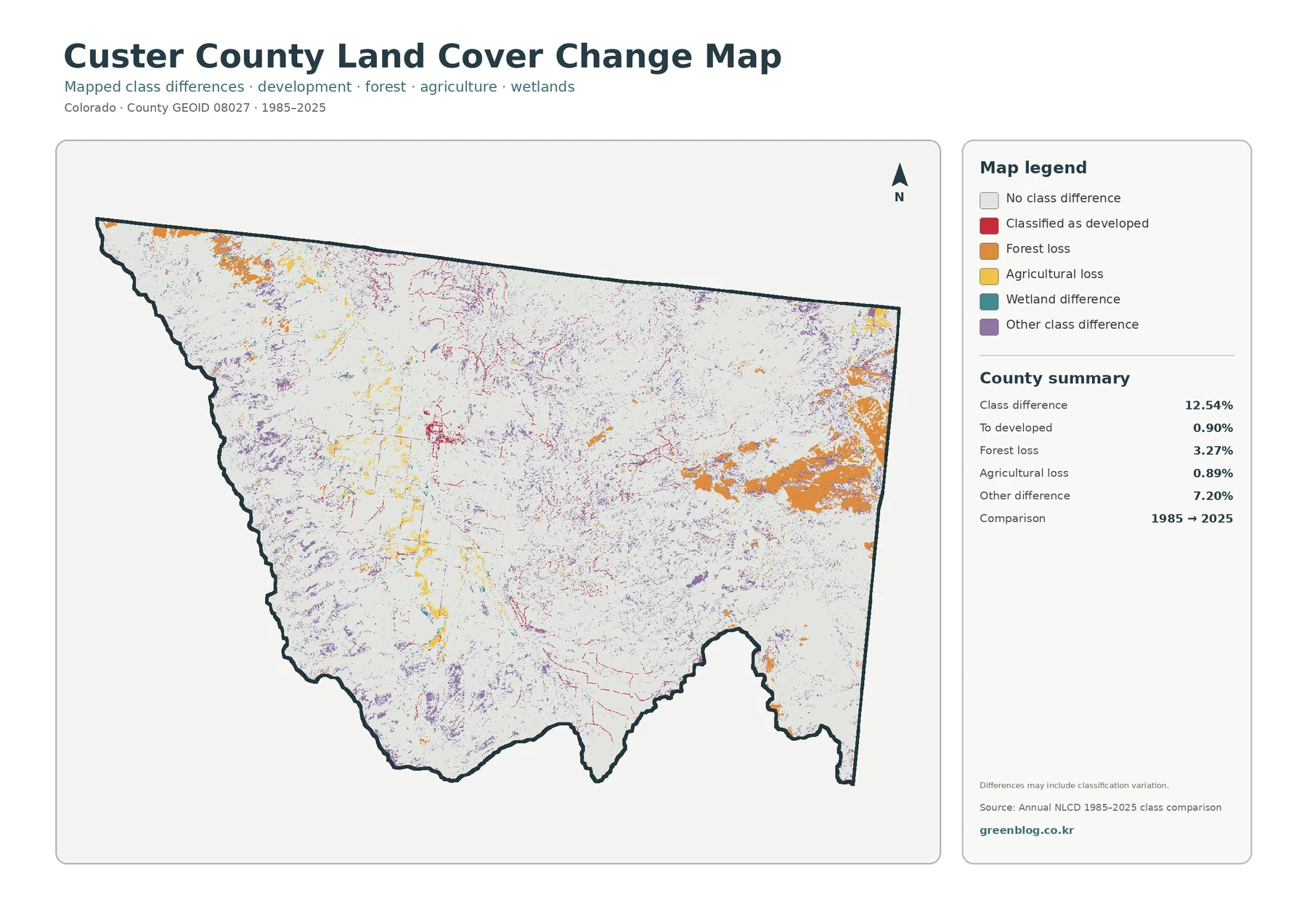
The change map compares the 1985 and 2025 classifications rather than showing the amount of every present-day cover type. A total of 12.54% is marked as a class difference. Within the summary, 0.90% is classified as change to developed, 3.27% as forest loss, 0.89% as agricultural loss, and 7.20% as other difference. The large “other difference” category is a reminder that the map should not be reduced to a single story about urban growth or forest decline.

Red change-to-developed marks are easiest to see around the central town area, with additional thin traces scattered elsewhere. Orange forest-loss areas are more noticeable in parts of the east and northeast, while smaller patches also occur along other mountain sections. Yellow agricultural-loss marks appear in parts of the central valley. Purple and other change colors are widely scattered. The locations show that different kinds of mapped change occur in different settings rather than forming one uniform band across the county.

A colored cell is not automatically evidence of one documented event on the ground. The map itself notes that differences may include classification variation. Forest and shrub boundaries, grass and agricultural edges, and other mixed landscapes can be classified differently when imagery or conditions change. Small isolated pixels deserve caution. Larger patches and repeated patterns are more useful for deciding where to investigate with additional aerial imagery, annual land-cover products, or local records.

The 40-year comparison works well as a starting point for follow-up research. Someone interested in development can begin with the central red cluster. A forest-focused study can examine the larger orange patches in the eastern highlands, while an agricultural study can trace yellow changes through the valley. The map does not establish why those changes occurred. Connecting a mapped difference to wildfire, timber activity, new construction, grazing, or another cause requires evidence from a separate source.

Use the same locations to compare all four views

The four maps become more informative when the same location is followed from one view to the next. Start in the central valley on the general land-cover map, where grass, shrub, agriculture, wetlands, and developed cover are all present. The forest and farmland view simplifies that mix and makes the open valley stand out against the mountain forests. The impervious map then isolates the compact built footprint near Westcliffe and Silver Cliff. Finally, the change map shows where change-to-developed and other class differences appear around the same part of the county.

The western Sangre de Cristo side offers a different comparison. Present-day maps show extensive forest, but the change map still contains scattered areas of forest loss and other class differences. The same is true on the eastern side, where current forest can coexist with mapped change over the 1985–2025 period. “Forested today” and “unchanged for forty years” are not equivalent statements. Keeping current condition and historical comparison separate prevents an easy misreading of the two products.

Water and wetlands provide another useful orientation cue. They cover small shares of the county, but their narrow shapes through the valley help align the maps visually. Once those features are located, nearby grass and agricultural patches can be compared more confidently. The impervious layer should not be expected to repeat those natural-cover colors because it answers a different question: how much hard surface is estimated within each cell. Choosing the map according to the question is more reliable than trying to read every theme from one image.

Choosing a map for printing, teaching, or regional reference

For a general overview, use the full land-cover map because it preserves the widest set of classes. It works well when the goal is to introduce the county’s forested mountains, open valley, wetlands, agricultural patches, and compact developed area in one image. If the discussion is specifically about forest versus open or agricultural land, the forest and farmland version is easier to read because several other classes are grouped or simplified.

The impervious map is the better choice for a presentation about built surfaces, settlement concentration, or watershed context. It clearly separates the small central developed footprint from the large low-impervious remainder of the county. For a history or change topic, the 1985–2025 map is more appropriate, but it should be presented with its classification caveat. A change class identifies a difference between mapped categories; it does not automatically provide a cause.

In a classroom or slide deck, the maps can be shown in sequence because they use the same county outline. A useful order is current land cover, forest and farmland, impervious surface, then long-term change. Students can first identify the valley and mountain forests, then compare human-made surfaces, and finally ask where classifications changed through time. This creates a geographic comparison without requiring the maps to function as legal land records or parcel-scale measurements.

Scale, classification, and what the maps cannot tell you

Every land-cover product represents conditions associated with a particular dataset year. The current maps in this package are labeled 2025, while the change view compares 1985 with 2025. A wildfire, construction project, vegetation shift, or water-level change after the observation period may not appear. When a current field condition matters, the map should be paired with more recent imagery or an official local source.

Raster generalization is another limitation. The landscape is divided into grid cells, and each cell receives a class or impervious estimate. Along a forest edge or a narrow wetland, one cell may contain several real-world surfaces. This produces mixed pixels and simplified boundaries. Enlarging the JPG does not create additional survey accuracy, so small color fragments should not be used as exact lines for property, wetland permitting, or infrastructure decisions.

Land cover is also different from land use and zoning. Forest, grass, water, and pavement describe what covers the ground. Zoning describes rules for how land may be used, while parcel data identifies property boundaries. Custer County’s official GIS page lists zoning, subdivision, conservation-easement, and other local mapping resources separately. That separation is a useful reminder to match the data source to the decision being made.

Frequently Asked Questions

Related Maps

• Adams County Colorado Land Cover Map
• Alamosa County Colorado Land Cover Map
• Arapahoe County Colorado Land Cover Map

Sources and References

• MRLC Annual NLCD Data – official access point for Annual NLCD land-cover products.
• USGS Annual NLCD Land Cover Classification – explains the classes used in the Annual NLCD product.
• Custer County, Colorado – official county information describing the Wet Mountain Valley, Westcliffe, and the Sangre de Cristo setting.
• Custer County GIS & Maps – official local mapping resources for zoning, subdivisions, conservation easements, and other subjects distinct from land cover.
• Custer County Hazard Mitigation Plan – official county context for the Wet Mountains, Wet Mountain Valley, DeWeese Reservoir, and local geography.
• U.S. Census Bureau TIGER/Line Shapefiles – official geographic boundary reference.