Alamosa County sits on the floor and eastern edge of Colorado’s San Luis Valley, where the 2025 land-cover map changes sharply from broad shrubland to irrigated fields, wetlands, a compact developed area around Alamosa, and forest along the eastern mountains. This page compares four views of the same county: general land cover, forest and farmland, impervious surface and developed land, and mapped class differences between 1985 and 2025.
The WebP images in the article are designed for quick viewing. The download section provides the four original JPG maps at 2480×1754 pixels in one ZIP. They are useful for comparing the farmed valley floor with the eastern uplands, locating wetland concentrations, separating road and building surfaces from agricultural grids, and identifying places where the mapped class changed between the two comparison years. These maps describe surface cover, not zoning, ownership, parcel boundaries, or development rights.
Table of Contents
A county dominated by shrubland but divided by very different landscapes
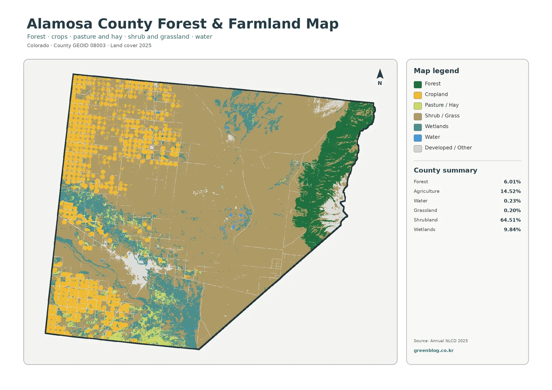
Shrubland is the dominant 2025 class at 64.51 percent, and its broad tan color fills much of the county. Agriculture accounts for 14.52 percent, wetlands 9.84 percent, forest 6.01 percent, and developed land 3.30 percent. Water is 0.23 percent and grassland is 0.20 percent. Those percentages give a useful summary, but the location of each class is just as important. Agriculture does not appear evenly across the county, forest is strongly concentrated on the east side, and development forms a much smaller but recognizable cluster near the city of Alamosa.
The western and southwestern parts of the map contain repeated yellow circles and rectangular fields. The regular shapes stand out against the surrounding shrubland and wetland colors and make the irrigated agricultural landscape easy to recognize. The map does not identify crops or individual farm ownership, so it should not be used to label a specific field. It does, however, show that farming is concentrated on the flatter valley floor rather than spread uniformly into the eastern mountain zone.
Wetlands form another important part of the county pattern. Teal areas appear through the lower western and southern portions of the county and in several interior patches, often close to agricultural cover. With 9.84 percent of the county classified as wetlands, they are too extensive to treat as a minor background class. Their distribution also helps explain why a simple description of Alamosa County as a dry valley misses a major part of what the map actually shows.
The official National Park Service description of Great Sand Dunes National Park and Preserve emphasizes the variety of the surrounding landscape, including grasslands, wetlands, forests, alpine environments, and the dune field. The park and preserve extend into Alamosa and Saguache counties. The county land-cover map is not a park-boundary map, but the strong shift toward forest and other natural cover on the east side fits the broader landscape contrast described by the NPS.
Irrigated fields on the valley floor and forest on the eastern edge
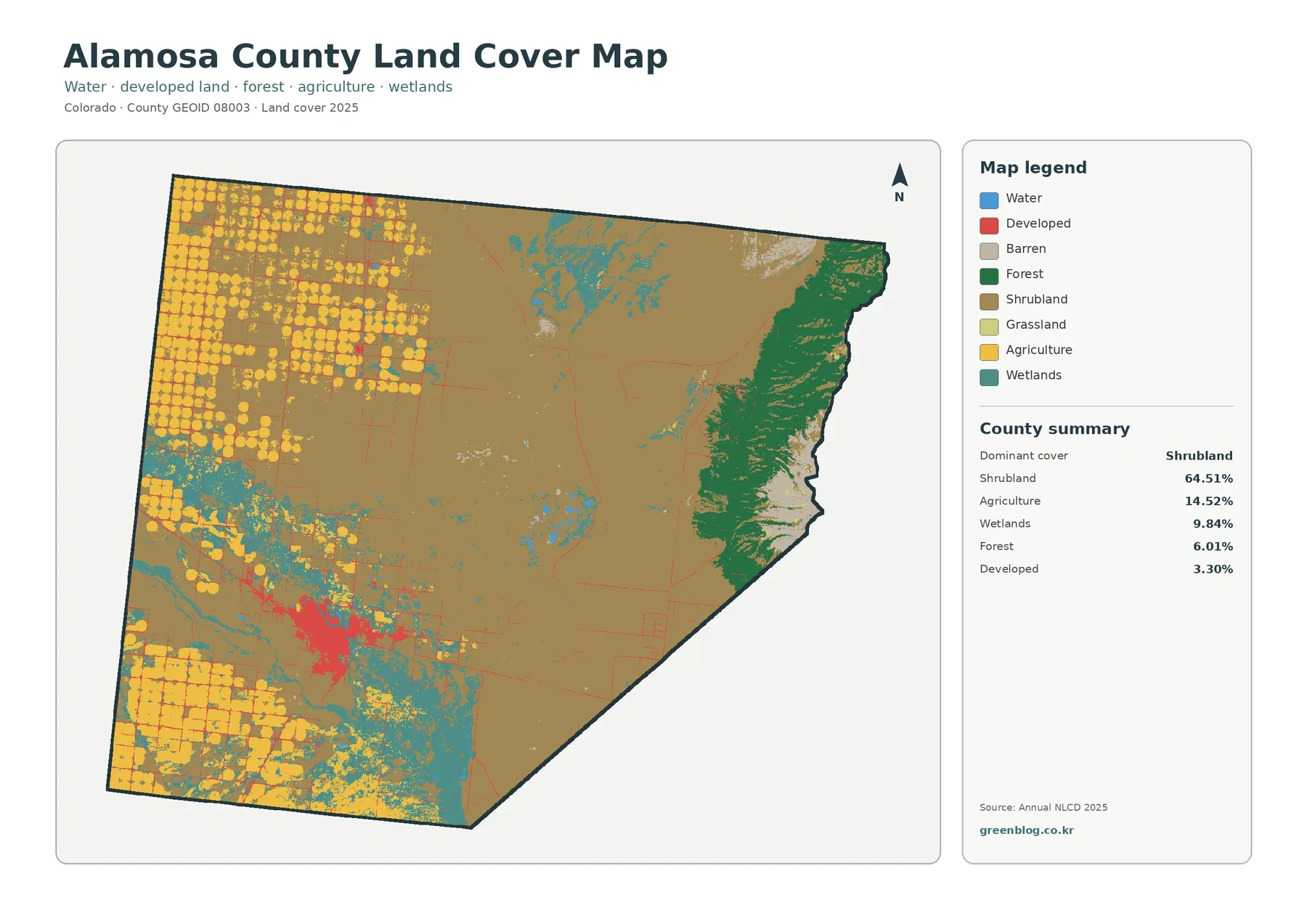
The forest and farmland view simplifies the county enough to make its east-west contrast especially clear. Dark green forest forms a long belt along the eastern boundary, while cropland is concentrated in the west and southwest. Between them lies a much larger area of shrub and grass cover, interrupted by wetlands and smaller developed or other classes. This map is useful when the full legend of the general land-cover map feels too busy and the main question is where agriculture and forest occur relative to one another.
The eastern forest does not cover the whole mountain-facing side with the same intensity. It is strongest in a broad band and is interrupted near lighter high-elevation or nonforest surfaces. That distinction matters because a green mountain edge should not be interpreted as a single uniform forest block. The map provides a generalized surface classification, so treeline, open slopes, roads, and other small features can be simplified at this scale.
Agricultural cover has a very different geometry. Circular irrigation patterns are prominent in the northwest, with additional blocks and circles toward the southwest. The visible organization of those fields is one of the most county-specific features in the package. It provides a clear contrast with the large central shrubland area, where field shapes become much less frequent. In a classroom or presentation, this single map can demonstrate how a broad valley can contain both intensive irrigated agriculture and large open areas within the same county.
Water occupies only 0.23 percent of the 2025 summary, but water-related land cover is more important than that number alone suggests because wetlands cover 9.84 percent. Colorado Department of Agriculture material about the San Luis Valley and Rio Grande headwaters describes the close relationship among agriculture, irrigation, wetlands, and watershed health. The county map should not replace a hydrology or irrigation map, yet the close placement of farmland and wetland colors provides a useful starting point for asking where more detailed water data may be needed.
Impervious surfaces reveal how compact the developed footprint is
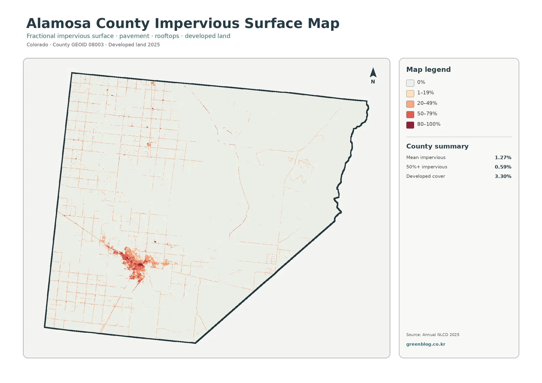
The impervious-surface map looks much lighter than the other three maps because hard surfaces occupy only a small share of the county. Mean imperviousness is 1.27 percent, and areas with at least 50 percent impervious cover account for 0.59 percent. Developed cover in the general land-cover summary is 3.30 percent. The darkest colors are concentrated around the city of Alamosa, while thin lines extend outward along roads and smaller built features.
Impervious surface means pavement, rooftops, and other surfaces where water does not easily soak into the ground. The percentage is mapped by cell, so a pale road corridor and a dark urban block represent different levels of hard-surface concentration. Around Alamosa, the connected red and orange pattern forms a clear urban core. Away from that core, most of the county returns quickly to very low impervious values, even where straight agricultural roads create a visible grid.
This map is particularly helpful for avoiding a common visual mistake. The agricultural landscape also contains many straight lines, but a field grid is not the same thing as a developed surface. Comparing the farmland map with the impervious map separates the large cultivated areas from the smaller network of pavement and buildings. That distinction is useful in watershed discussions, transportation context, and basic urban-growth comparisons.
Imperviousness should not be treated as a flood-risk score. Runoff depends on slope, soil, drainage infrastructure, rainfall intensity, channels, and other conditions that are not shown here. The safe interpretation is narrower: the map identifies where hard surfaces are concentrated and how limited their overall footprint is relative to the county’s shrubland, agricultural land, wetlands, and mountain cover.
Where the 1985 and 2025 classifications differ
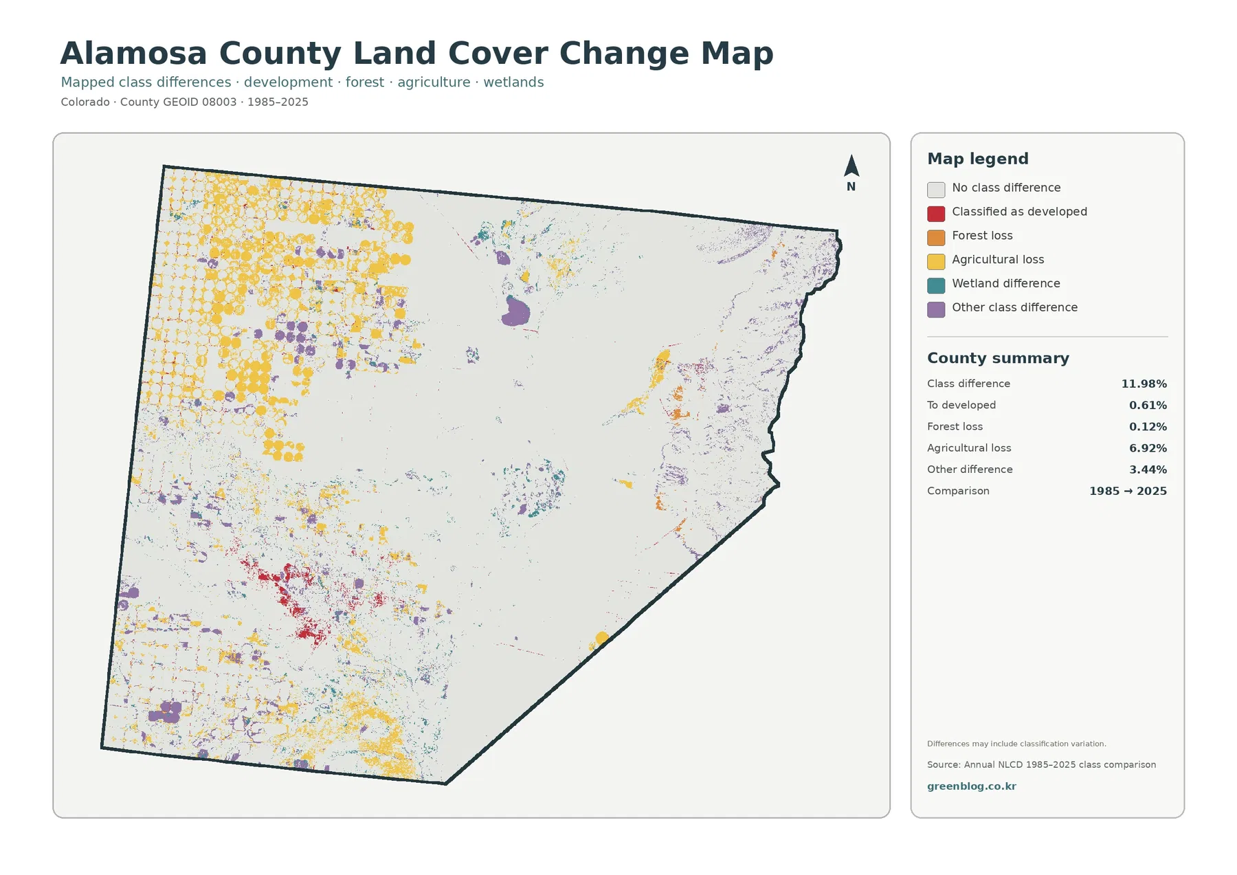
The change map compares the mapped class in 1985 with the class in 2025. A total of 11.98 percent of the county is marked as a class difference. The summary identifies 6.92 percent as agricultural loss, 0.61 percent as classified to developed, 0.12 percent as forest loss, and 3.44 percent as other class difference. Wetland difference also has its own legend color, so the colored pattern on the map provides information that cannot be reduced to a single headline percentage.
Yellow agricultural-loss symbols are especially visible in the northwestern field area and in parts of the south. They often follow the same circular and rectangular field geometry seen on the 2025 farmland map, but they do not cover every agricultural parcel. Purple other-class differences are scattered among some of those fields and appear in several interior locations. Around the Alamosa urban area, red pixels indicating classification to developed are more concentrated than in the rest of the county.
The eastern side has much less change color overall, although small patches of forest loss and other differences appear along the mountain-facing zone. This is a good example of why the countywide 11.98 percent figure needs a map. The same percentage could result from a uniform pattern or from several localized clusters, and Alamosa County clearly shows the latter. The northwest, urban southwest, interior wetland areas, and eastern edge do not share the same type or density of change.
A class difference is not automatically proof of permanent land conversion. Annual NLCD comparisons can capture real surface change, but they can also be affected by classification methods, imagery conditions, mixed pixels, and small boundary shifts. The map itself notes that differences may include classification variation. For a specific farm, wetland, road project, or forest patch, use this layer to identify a place worth checking and then verify it with dated aerial imagery, local records, or field information.
Reading the four maps as one county story
The four views answer different parts of the same geographic question. The general land-cover map establishes the dominant 64.51 percent shrubland background and shows where agriculture, wetlands, forest, and development fit within it. The forest and farmland view removes some legend complexity so the western agricultural area and eastern forest belt are easier to compare. The impervious map isolates the built footprint, and the change map shifts attention from current condition to places where the two classification years disagree.
Around Alamosa, those layers become especially useful together. The general map places the developed cluster among wetlands, agriculture, and shrubland. The impervious map sharpens that cluster into a concentration of roads, buildings, and other hard surfaces. The change map adds red areas classified to developed in and around the same broader urban zone. The maps support a statement that these patterns occur near one another, but they do not by themselves prove that one land-cover type caused the loss of another.
The east side tells a different story. Forest is prominent there in the 2025 maps, while cropland largely disappears. The change layer contains relatively small and scattered differences compared with the agricultural northwest. Because Great Sand Dunes National Park and Preserve reaches into Alamosa County and the NPS describes a landscape that includes forests, wetlands, grasslands, dunes, and alpine environments, the eastern portion is a useful place to pair the land-cover image with official park information. The county map still should not be used as a substitute for the NPS boundary map.
The wetland pattern is the third major thread connecting the maps. Wetlands occupy 9.84 percent of the 2025 summary, appear in complex patches among the western and southern valley floor, and receive a separate difference class on the change map. A reader interested in habitat, water management, or irrigation can use those locations to guide more detailed research. The land-cover map identifies where surface classes appear; it does not provide water depth, seasonal duration, ownership, or legal water rights.
Practical uses for printing, teaching, and preliminary comparison
The four original JPG files are 2480×1754 pixels. That size works well for on-screen reference, reports, slide decks, and many ordinary print layouts. The asset manifest does not mark them as meeting the package’s A3 high-resolution reference, so anyone planning a full-page A3 print should test a sample first and check whether the legend and fine field patterns remain readable at the intended scale. Keeping the original dimensions avoids quality loss from unnecessary enlargement and re-encoding.
For teaching, a useful sequence is to begin with the general map and ask students to identify the dominant class, then switch to the forest and farmland view to locate the strongest east-west contrast. The impervious map can introduce the difference between an agricultural grid and a built surface. Finally, the change map can lead into a discussion of why a two-date classification comparison needs verification before it is described as a confirmed land-use change.
For environmental or planning context, the maps work best as screening and communication tools. A watershed project might use the wetland and impervious maps to identify areas where more detailed runoff or habitat information is needed. A county presentation could use the agriculture and forest map to explain why one description of the whole county is inadequate. A historical comparison could use the change layer to select locations for aerial-photo review. None of those uses require treating the map as parcel-level evidence.
The maps are also useful for general regional orientation because the county contains a visually strong transition from valley floor to eastern uplands. The NPS describes Great Sand Dunes as part of a diverse landscape rather than an isolated dune field, and the land-cover maps reinforce that point by showing wetlands, shrubland, forest, agriculture, and developed areas within the same county. That diversity is one reason Alamosa County benefits from having several map views instead of a single simplified graphic.
Limits that matter before using the data
Annual NLCD is a raster classification, meaning the landscape is represented by a grid of cells. A cell can contain more than one real-world surface, so the assigned class is a generalized representation rather than a surveyed boundary. Edges between a wetland and a field, or between forest and open land, may therefore look cleaner on the map than they are on the ground. Mixed pixels become particularly important along narrow roads, small streams, field margins, and patchy vegetation.
The 2025 map is tied to its observation and classification year. Construction, agricultural rotation, restoration, wildfire, drought effects, or other changes after that year may not appear. The 1985–2025 comparison is even more limited in one respect: it compares two endpoints and does not show every step in between. A place may have changed more than once during those four decades without that sequence being visible in the final two-date category.
County boundaries are included to give the land-cover data a clear administrative frame. Census TIGER/Line data are a standard source for such boundaries, but this page is not a legal survey. Parcel lines, easements, ownership, zoning, tax status, and development permission require separate authoritative records. Keeping that distinction clear allows the maps to do what they do well: show broad patterns and contrasts across Alamosa County without implying precision they were not designed to provide.
Download the Alamosa County map files
The download ZIP contains the four original JPG maps used in this article: general land cover, forest and farmland, impervious surface and developed land, and the 1985–2025 land-cover change comparison. Each image is 2480×1754 pixels. The article previews are WebP files for web display, while the downloadable JPGs are the original map exports supplied by the package.
Frequently Asked Questions
What is the dominant land-cover class in Alamosa County?
Shrubland is the largest 2025 class at 64.51 percent. Agriculture follows at 14.52 percent and wetlands at 9.84 percent, with forest at 6.01 percent and developed land at 3.30 percent. The spatial pattern matters as much as the totals: agriculture is concentrated in the west and southwest, forest along the eastern edge, and development around Alamosa.
Which map is best for seeing the built-up area around Alamosa?
The impervious-surface map is the clearest choice because it isolates pavement, rooftops, and similar hard surfaces. Mean imperviousness is only 1.27 percent countywide, but the darker colors are strongly concentrated in the Alamosa urban area. Pair it with the general land-cover map when you also want to see nearby agriculture, wetlands, and shrubland.
Does every colored area on the 1985–2025 map represent confirmed land conversion?
No. The layer shows locations where the mapped class differs between 1985 and 2025. Some differences can reflect real change, while others may be influenced by classification variation, imagery, mixed pixels, or boundary shifts. Use the map to locate areas for follow-up and verify a specific site with dated imagery or local records before drawing a firm conclusion.
Map File Information
Download the four original Alamosa County land-cover JPG maps together in one ZIP file.
- Printable Size: 2480×1754 pixels each
- File Type: ZIP containing four JPG files
Related Maps
Sources and further reading
- MRLC Annual NLCD Data – official access point for Annual NLCD land-cover products.
- USGS Annual NLCD Land Cover Classification – class definitions and interpretation guidance.
- U.S. Census Bureau TIGER/Line Shapefiles – county boundary reference data.
- Colorado.gov: Alamosa County – official state directory page for the county.
- Great Sand Dunes National Park & Preserve – official NPS information on the park, preserve, and surrounding landscape in Alamosa and Saguache counties.
Green Map creates custom-edited map images using open geographic data sources such as geoBoundaries, Natural Earth, OpenStreetMap, and government open data.
These maps are edited visual materials, not raw data files, and are provided for education, documents, presentations, and graphic reference.