Costilla County’s 2025 land-cover picture is dominated by shrubland and forest rather than built surfaces. Shrubland accounts for 57.91% of the mapped area, while forest covers 26.08%. The broad contrast is visible immediately: large shrub-covered areas occupy much of the west and center, and a substantial forested zone runs through the eastern side. This page explains that pattern with four map views and provides the original JPG set in one download.
The four maps separate questions that are easy to mix together on a single image. One shows the complete 2025 land-cover classification, another simplifies the view around forest and farmland, a third isolates impervious surfaces such as pavement and rooftops, and the last compares mapped classes in 1985 and 2025. They describe surface cover, not property ownership, zoning, parcel boundaries, or legal development rights.
Table of Contents
A county split between broad shrubland and eastern forest
The county summary lists shrubland at 57.91%, forest at 26.08%, agriculture at 4.96%, grassland at 4.93%, and developed land at 2.09%. The forest-and-farmland view also reports wetlands at 2.05% and water at 0.10%. These figures make the main landscape balance clear: shrubland is the largest class by a wide margin, but forest is concentrated enough to form a distinct eastern block rather than appearing as scattered fragments everywhere.
Agricultural cover has a different geometry. It appears in clusters of bright, often block-shaped parcels in the west-central part of the county and again farther south. Grassland and wetland classes are more dispersed. Developed cover is present but occupies a small share of the county, so the broad map is visually controlled by natural or semi-natural cover rather than by a continuous built area.
The 2025 land-cover map gives the broadest comparison
The general land-cover map is the best starting point because it keeps every major class in view. Brown shrubland covers most of the western half and extends through the center. Dark green forest becomes much more prominent to the east and northeast, with additional forested areas extending southward along the eastern side. Yellow agricultural patches form several separate groups instead of one continuous farming belt.
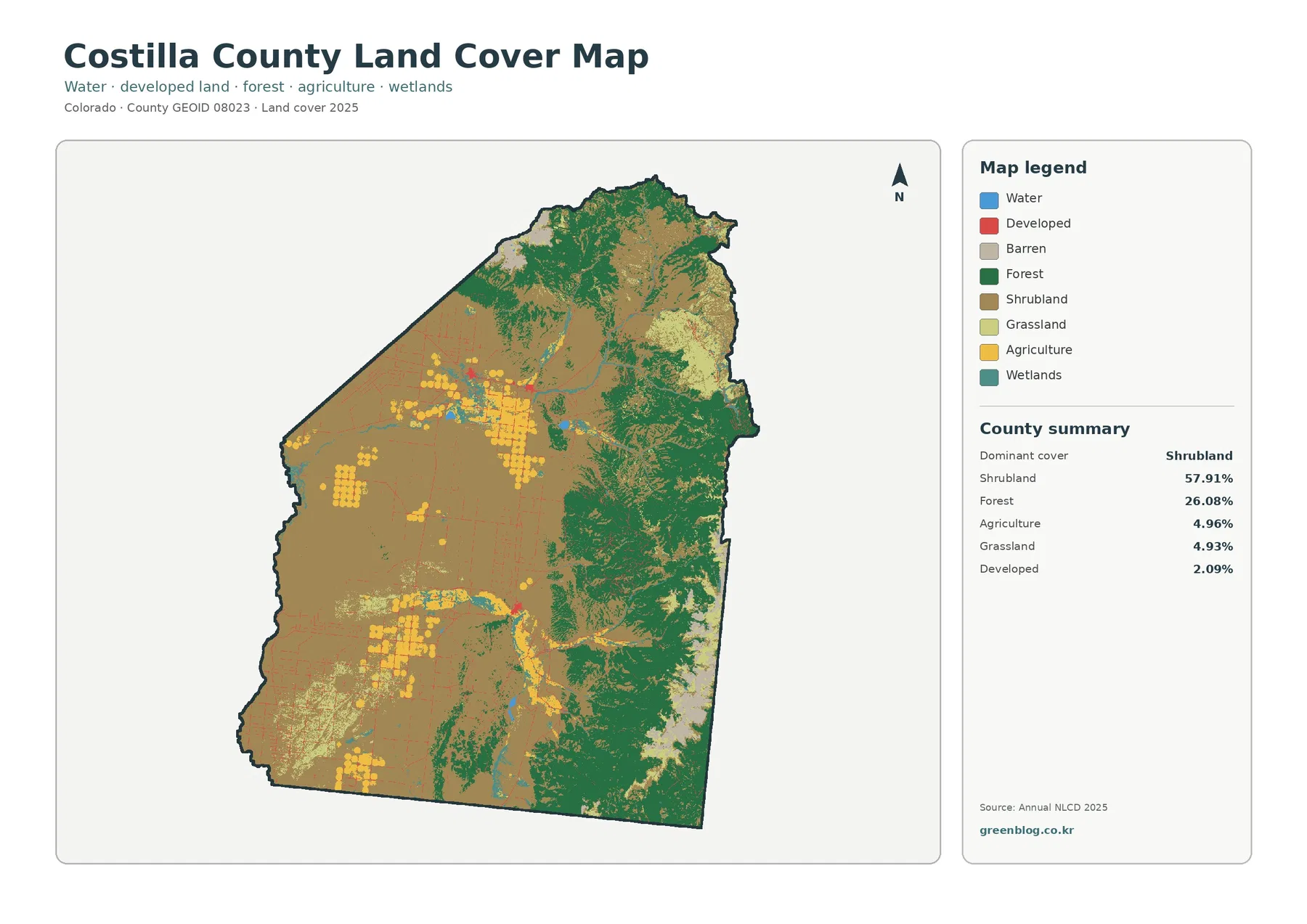
Wetland and water classes are much smaller in area, but they are easier to see when location matters more than percentage. Water represents only 0.10% of the county summary, while wetlands account for 2.05%. Their mapped patches and narrow areas should not be treated as a legal wetland inventory or a current water-level map. They are land-cover classifications within the dataset used to make the county map.
Built surfaces are sparse when viewed on their own
The impervious-surface view provides useful context for the 2.09% developed-cover figure. Average imperviousness is just 0.36%, and only 0.02% of the county is shown at 50% impervious or higher. Most of the map is therefore very pale, while stronger orange and red values appear only in small concentrations and thin lines.
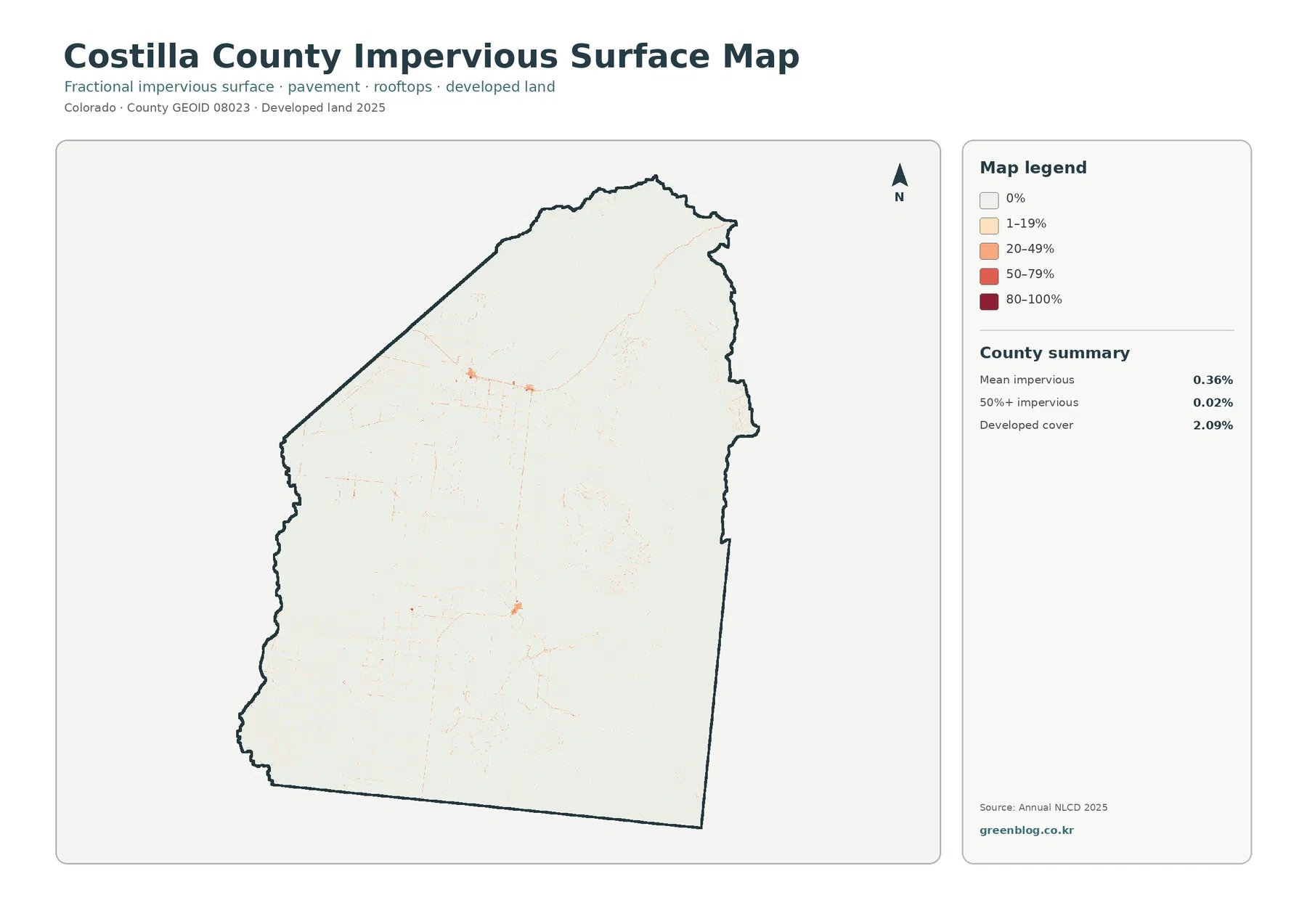
This map is useful when the red developed class on the general map needs closer interpretation. A developed land-cover class does not mean that every cell is covered by pavement or buildings. The impervious layer instead emphasizes how much hard surface is present within mapped cells. In Costilla County, the low countywide average confirms that concentrated built surfaces occupy only a very small portion of the mapped area.
The preview does not label individual roads or settlements, so the bright locations should not be assigned names from the image alone. What can be stated confidently is their pattern: higher impervious values form small nodes and narrow connections rather than a large continuous urban field. That distinction matters when comparing Costilla County with more intensively developed counties.
Forest and farmland become easier to compare in the simplified map
Removing some of the general-map complexity makes the east-west contrast even clearer. Forest remains concentrated on the eastern side, while shrub and grass cover fills much of the west and center. Cropland and pasture or hay appear as brighter blocks and smaller bands embedded within that broader open cover.
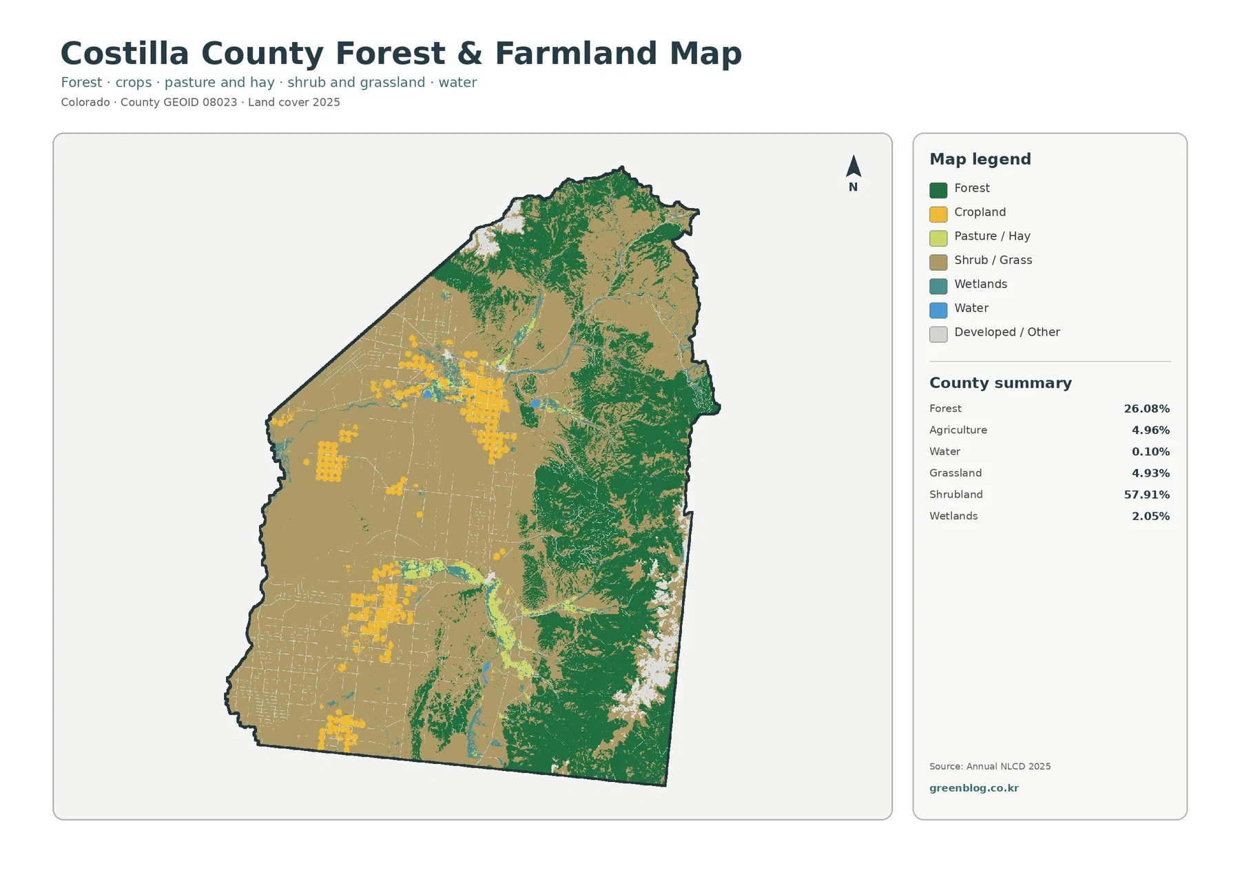
Agriculture totals 4.96% in the county summary, yet its regular shapes make it visually prominent in several places. The largest clusters are not spread evenly across the county. They are grouped in the west-central area and again in the southern interior, with smaller patches elsewhere. This is a good example of why percentages and map position should be read together: a class can have a modest countywide share but still be locally important where it is concentrated.
Grassland represents 4.93%, close to the agricultural share, but it does not appear in the same block-like pattern. Wetlands at 2.05% are smaller still and occur as patches or narrow features within the broader mix. Those classes can be useful for environmental education or regional comparison, but the map should not be used to identify a parcel-level wetland boundary or to decide how a specific property may be managed.
Mapped differences from 1985 to 2025 are widespread but not uniform
The change map compares classifications in 1985 and 2025 rather than showing the 2025 composition again. Its county summary reports a 14.71% class difference. Within that total, 0.73% is classified as change to developed land, 4.02% as forest loss, 1.65% as agricultural loss, and 8.08% as other class difference. These figures are change categories, so they should not be confused with the 2025 shares of forest, agriculture, or developed land.
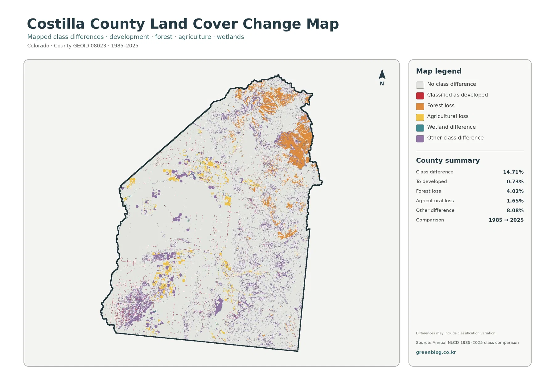
Orange forest-loss classifications are especially noticeable in the north and northeast and along portions of the eastern side. Purple other-difference areas appear in several western, central, and southern locations, while yellow agricultural-loss classifications are more localized around areas that also contain present-day agriculture. Red change-to-developed pixels are visible but occupy a small share overall.
The map itself warns that differences may include classification variation. That note is important. A changed class does not by itself establish a cause, prove land degradation, or identify a particular development event. Satellite-based classification can differ because the surface truly changed, because mixed land-cover signals were assigned differently, or because conditions at the observation dates affected the classification. The map is most useful for locating places that deserve closer comparison, not for declaring why they changed.
A practical way to read all four maps
Start with the general 2025 map and identify the dominant cover. In Costilla County, that means recognizing the broad shrubland area first and then the large eastern forest zone. Next, use the forest-and-farmland map to separate agriculture, grassland, wetlands, and forest more clearly. This sequence keeps small but meaningful classes from being lost in the busier legend of the complete map.
Move to the impervious map only after locating developed cover on the first image. The 0.36% mean impervious figure helps distinguish a small developed classification from a heavily hard-surfaced landscape. Finally, compare the change map with the current maps. A place that is forested in 2025 may still contain mapped change since 1985, and a shrubland-dominated area may include several kinds of historical class difference. Current condition and change history answer different questions.
For presentations, that sequence can also reduce confusion. Use the full land-cover map to introduce the county, the forest-and-farmland view for a land-management or agriculture discussion, the impervious map for built-surface context, and the change map when the topic is comparison across time. Each image is more useful when it is paired with the question it was designed to answer.
Ways the map set can be used
In a classroom, the county provides a straightforward example of how a dominant class can coexist with strong local contrasts. Students can begin with the 57.91% shrubland figure, find the broad western and central areas that correspond to it, and then compare that with the 26.08% forest share concentrated in the east. Agriculture provides a second lesson because its 4.96% share forms visible clusters rather than a uniform layer.
For county-to-county comparison, the same statistics can be used as reference points as long as the compared maps use the same classification year and system. The impervious layer is particularly useful in that setting because a developed-cover percentage and an impervious percentage describe related but different characteristics. In Costilla County, developed cover is 2.09%, while average imperviousness is only 0.36%.
Environmental or watershed-oriented work can use the wetland and water classes to identify broad locations for further study, but the maps should remain a screening and communication tool. They do not replace current field observations, engineering data, legal wetland determinations, parcel records, or local planning documents. The same caution applies to the change map: it can guide where to look more closely, but it cannot establish the cause of a mapped difference.
What the maps do not show
These are raster land-cover maps, meaning the landscape is represented as classified cells rather than surveyed parcel polygons. A cell can contain more than one real-world surface, and a single class may be assigned even when several surfaces are present. Narrow roads, small buildings, small water features, or thin wetland areas may therefore be simplified. The preview package does not state a parcel-level precision standard, so none should be assumed.
Time is another limitation. The current maps are labeled 2025, while the comparison map spans 1985 to 2025. Changes that occurred after the observation period will not appear, and the exact appearance of a class can vary between years. For that reason, the 14.71% class-difference figure should be described as mapped classification difference, not as 14.71% of the county being damaged, developed, or permanently converted.
The downloadable JPGs preserve the map information supplied in this package at 2480×1754 pixels. A larger on-screen zoom may make labels and class boundaries easier to inspect, but it does not create new source detail. Use the maps for county-scale comparison and communication, then consult more specific official data when a decision depends on exact boundaries or current site conditions.
Download the Costilla County land-cover JPG set
The ZIP below contains four original JPG maps: the 2025 land-cover map, forest-and-farmland map, impervious-surface/developed-land map, and the 1985–2025 land-cover-change map. Each original JPG in the supplied package is 2480×1754 pixels. The files are suitable for viewing, classroom use, reference graphics, and presentation layouts where county-scale patterns are the main purpose.
Frequently Asked Questions
What is the largest land-cover class in Costilla County?
Shrubland is the largest 2025 class at 57.91%. Forest is second at 26.08%. On the map, shrubland covers much of the west and center, while forest is concentrated mainly across the eastern side.
Does the 2.09% developed figure mean 2.09% of the county is pavement or rooftops?
No. Developed land cover and impervious surface are not the same measure. The impervious map reports a countywide mean of 0.36%, with only 0.02% mapped at 50% impervious or higher. Developed classes can include areas that still contain vegetation or other permeable surfaces.
Does the 14.71% class difference represent confirmed land loss?
No. It represents mapped classification differences between 1985 and 2025. The map notes that classification variation may be included, so the figure should be used to locate and compare changes rather than to assign a cause or legal meaning.
Map File Information
The ZIP includes four original Costilla County land-cover JPG maps in one file.
- File Type: Four JPG files in one ZIP archive
Related Maps
- Adams County Colorado Land Cover Map
- Alamosa County Colorado Land Cover Map
- Arapahoe County Colorado Land Cover Map
Sources and Data References
- MRLC Annual NLCD Data — official access point for the Annual NLCD data family used for land-cover analysis.
- USGS Annual NLCD Land Cover Classification — official explanation of land-cover classes and classification terminology.
- U.S. Census Bureau TIGER/Line Shapefiles — official boundary and geographic-unit reference data.
Green Map creates custom-edited map images using open geographic data sources such as geoBoundaries, Natural Earth, OpenStreetMap, and government open data.
These maps are edited visual materials, not raw data files, and are provided for education, documents, presentations, and graphic reference.