Los Angeles County California Land Cover Map: Why the Urban South and Shrubland North Look So Different

The Los Angeles County California Land Cover Map brings together two landscapes that are easy to think of separately: one of the country’s largest continuous urban areas and a much broader county boundary filled with mountains, shrub-covered uplands, open northern terrain, reservoirs, and offshore islands. The 2025 summary lists shrubland at 49.69%, developed cover at 33.98%, grassland at 10.91%, forest at 3.05%, and agriculture at 0.87%.

Four map views are available here, and the four original JPG files can be downloaded together in one ZIP. The set includes general land cover, forest and farmland, impervious surface and developed land, and a 1985–2025 land-cover change comparison. These maps classify physical surface cover; they do not show parcel ownership, zoning, legal land use, or development entitlement.

The urban south is visually dominant even though shrubland is the largest countywide class

The first impression of the general map is the enormous red developed area across the southern mainland. Dense urban cover stretches from the central basin toward the coast and inland valleys, creating a nearly continuous footprint in the part of the county most people associate with Los Angeles. Yet that visual concentration covers a smaller countywide share than shrubland because the northern and mountain portions of the county are so extensive.

Shrubland, at 49.69%, fills much of the northern interior, major mountain belts, and western coastal uplands. It also threads through gaps near developed valleys. The class represents shrub-dominated surface cover rather than empty land. That distinction is important in Los Angeles County because large natural areas sit remarkably close to urban neighborhoods without becoming part of the continuous red developed footprint.

Grassland accounts for 10.91% and forms a lighter layer between the dominant classes. It is common in the northern county and along mountain margins, where it mixes with shrubland rather than forming one uninterrupted block. The land-cover class says nothing about whether a grass-covered site is a ranch, open-space preserve, public land, or privately held property.

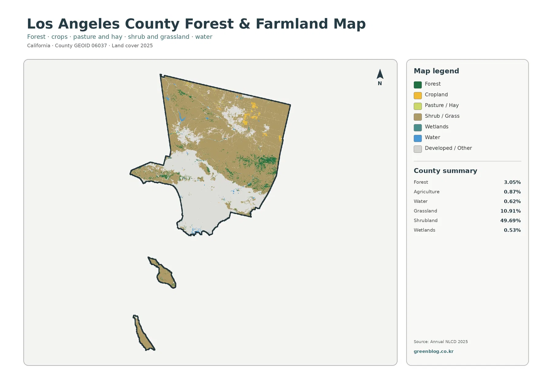
Forest covers only 3.05%, but its green patches are geographically distinctive. The most noticeable forest areas lie in mountain terrain through the central and eastern mainland, with smaller concentrations elsewhere. Those patches help separate broad shrub-covered mountains from the densely developed basin and from the more open Antelope Valley to the north.

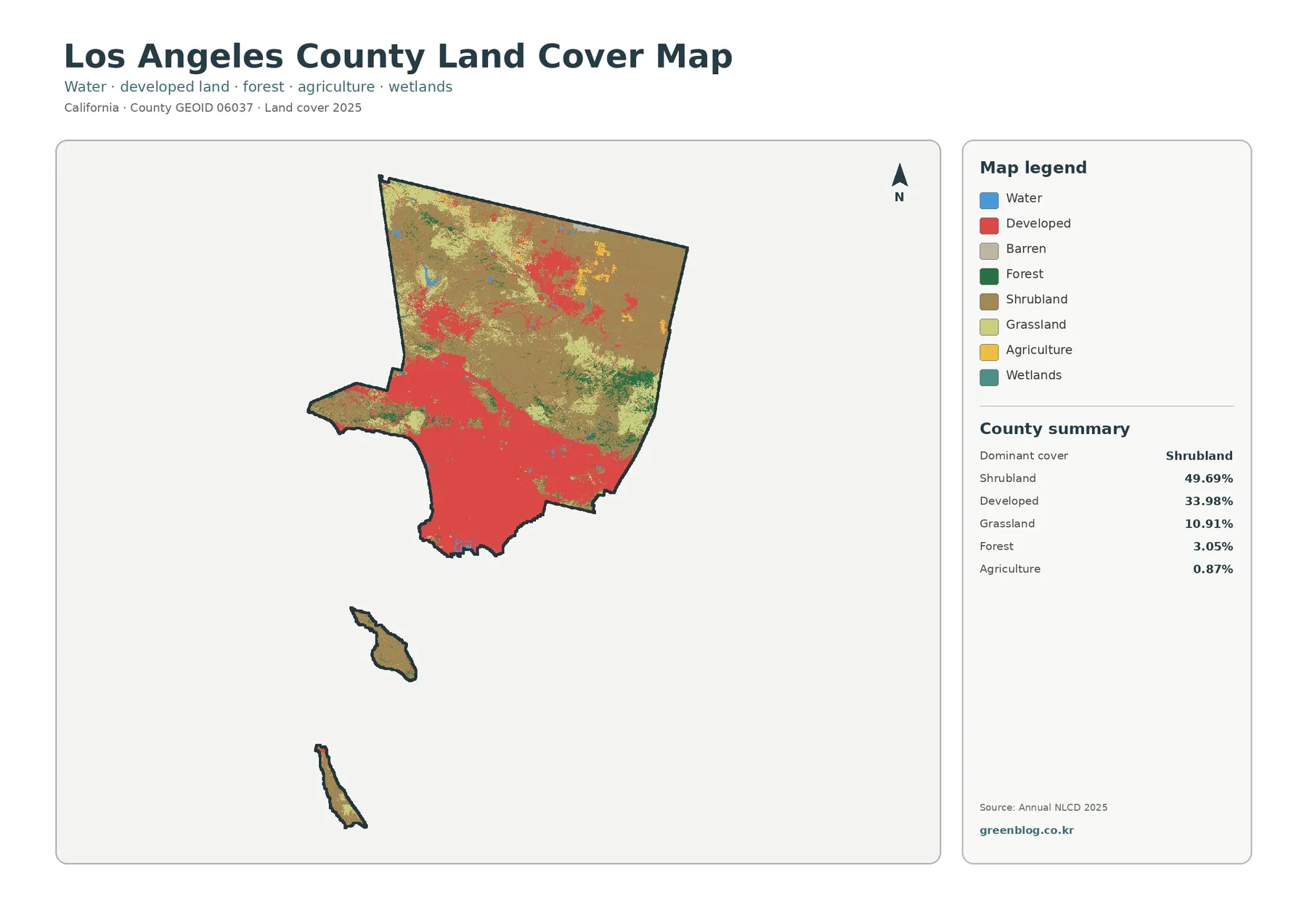
Reading the map from south to north is more useful than memorizing the legend first. The dense metropolitan red gives way to mountain shrubland and forest, then to a northern landscape where shrub and grass cover dominate around separate urban clusters. That sequence captures the county’s internal contrast in a way a single percentage cannot.

Antelope Valley development appears as separate islands of hard surface on the mainland

The northern portion of the county contains several visible developed clusters, but they are separated by broad shrubland and grassland. This is very different from the southern metropolitan footprint, where development is much more continuous. LA County Planning treats Antelope Valley as its own planning area, which provides useful local context for a northern landscape that has a distinct settlement pattern and much larger open areas.

The impervious map makes that difference even sharper. Hard surfaces in the north appear as compact red-orange groups surrounded by pale land, while the southern half contains an extensive network of high values. The contrast shows why developed cover and urban form should be discussed spatially rather than only through the countywide 33.98% figure.

A similar urban-natural boundary appears along the Santa Monica Mountains in the west. The mountains remain largely shrub-covered even though dense development lies immediately nearby. LA County Planning’s Santa Monica Mountains North Area Plan focuses on biological-resource protection and development regulation in unincorporated mountain communities, giving a planning context for this unusually close contact between natural cover and metropolitan land.

The impervious map separates a developed landscape from the surfaces that are actually paved or roofed

Los Angeles County has a mean impervious value of 18.33% in 2025, and 21.53% of the county is mapped at 50% or greater imperviousness. Developed cover is much larger at 33.98%. These numbers are not contradictory: a developed land-cover cell can include trees, yards, soil, and landscaped space, while impervious data estimate the share occupied by hard surfaces such as roofs and pavement.

The highest impervious values form a broad, connected mass across the southern mainland. Dark red extends through the central basin, coastal urban area, and inland developed corridors. Mountain ridges and shrub-covered slopes create obvious breaks, which helps reveal topographic barriers that are less apparent when looking only at county boundaries.

North of the mountains, the pattern becomes discontinuous again. The Antelope Valley clusters are clearly visible, yet huge areas around them remain nearly white. The result is a map where the same county contains both intensely hardened urban surfaces and vast areas with almost no mapped impervious cover.

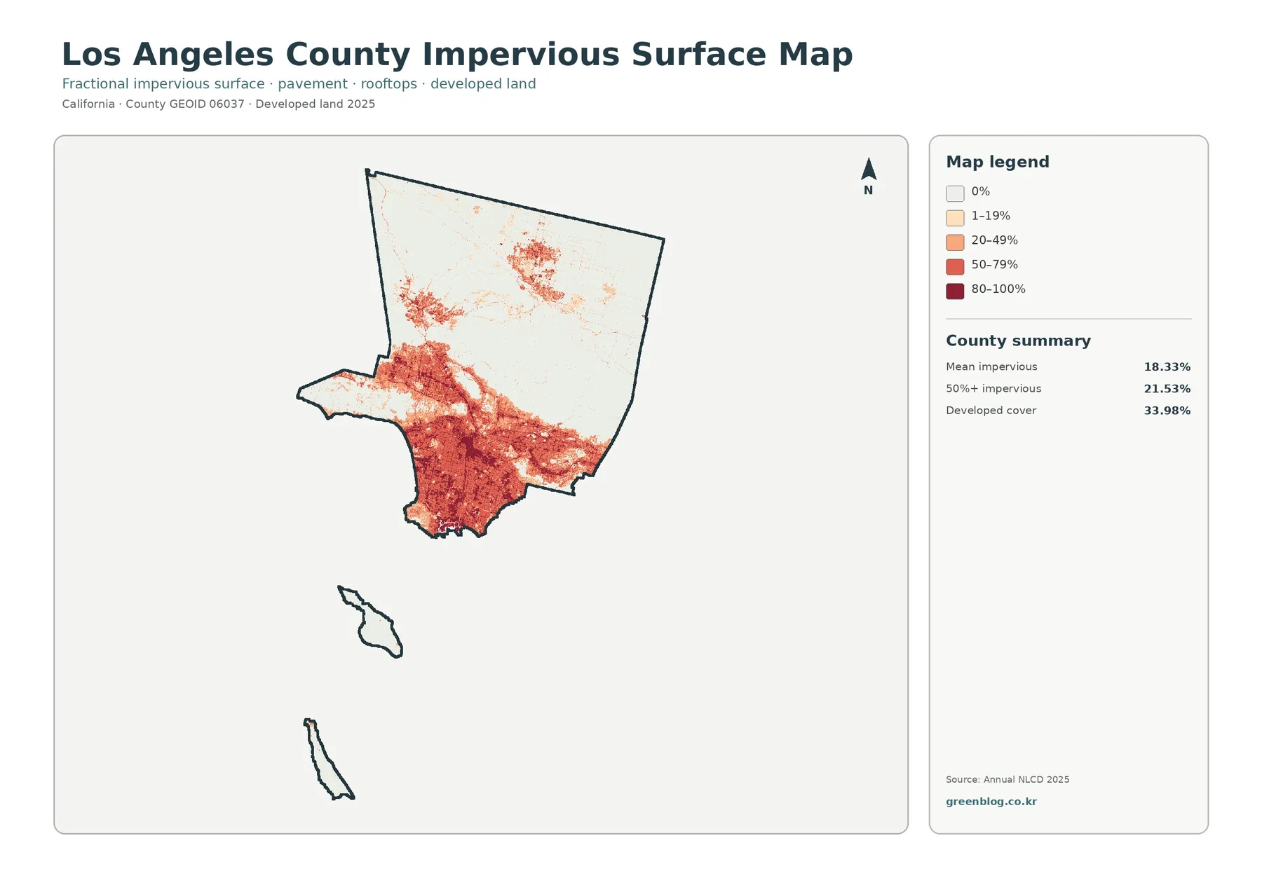
A county mean should never be used as the pavement percentage for a neighborhood or city. It averages the dense urban south with mountain, shrubland, grassland, and island surfaces that contribute very little impervious cover. Stormwater or flood analysis would also require rainfall, drainage, slope, soils, and channel data rather than this map alone.

A simplified natural-cover view makes the mountain belts easier to follow

The forest-and-farmland map removes much of the detail inside the developed classes and emphasizes the natural landscape. Shrubland remains 49.69%, grassland 10.91%, forest 3.05%, agriculture 0.87%, water 0.62%, and wetlands 0.53%. Southern development becomes a broad gray field, allowing the mountain and northern vegetation to stand out more clearly.

Forest is concentrated in portions of the central and eastern mountains, where green patches interrupt a much larger shrubland matrix. The western coastal mountains are more shrub-dominated. This difference is useful when discussing the county’s open space because “natural cover” is not a single uniform category: wooded slopes, chaparral-like shrub cover, and grass-dominated openings occupy different places.

Agriculture is only 0.87% and appears in a few northern and northeastern patches. The small share is notable in a county of this size, but it should not be interpreted as an agricultural production statistic. It simply records the cells classified as agricultural cover in the supplied 2025 dataset.

Water and wetlands also occupy small countywide shares. Inland reservoirs and lakes appear as blue points or patches, while wetland color is much more limited. A roughly 30-meter raster classification can simplify narrow channels and wetland margins, so the image is best used to locate broad aquatic areas rather than to establish regulatory boundaries.

The offshore islands repeat the county’s natural-cover story without the mainland’s urban intensity

Two offshore islands are drawn inside the county map, and both look very different from the southern mainland. Shrub and grass colors dominate the general view, while the impervious map remains mostly pale. The larger island is part of the county’s Coastal Islands planning framework; LA County Planning’s map catalog includes a Santa Catalina Island Local Coastal Plan map.

The islands are useful visual checks because they show that county land-cover statistics combine physically separate places. A dense mainland city block and an offshore shrub-covered slope both contribute to the same county summary. That makes location as important as percentage when interpreting a county with such varied geography.

On the mainland, the Santa Monica Mountains create a comparable break in urban continuity. Their shrub-covered slopes remain relatively light on the impervious map despite lying next to the metropolitan area. LA County’s Conservation and Natural Resources Element addresses open space, habitat, water, and scenic resources, a policy context that is distinct from the satellite classification but useful for understanding why these natural areas receive separate planning attention.

The 1985–2025 comparison concentrates change across mountains and expanding developed edges

Total mapped class difference between 1985 and 2025 is 25.17%. Other class difference is the largest category at 13.20%, followed by forest loss at 7.21%, transition to developed land at 4.09%, and agricultural loss at 0.60%. These numbers describe two-date classification differences; they are not a record of one permanent process affecting a quarter of the county.

Purple other-difference cells are widespread across northern and mountain terrain. Boundaries among shrubland, grassland, barren cover, and sparse vegetation can shift when vegetation condition, image timing, or classification behavior changes. The category is intentionally broad, so a purple patch should be treated as a location that deserves follow-up rather than as evidence of a specific event.

Forest-loss cells, mapped in orange, are especially noticeable through mountain areas. Some may represent real vegetation disturbance, but fire, drought, regrowth stage, image conditions, and classification changes can all influence a two-date result. Intermediate Annual NLCD years and fire or forest records are necessary before assigning a cause.

Red transition-to-developed cells tend to occur around existing urban areas and at some metropolitan edges. Comparing them with the 2025 impervious map helps show where long-term classification change overlaps with today’s hard-surface concentrations. The 4.09% value is not an annexation total, building-permit acreage, or zoning-change measure.

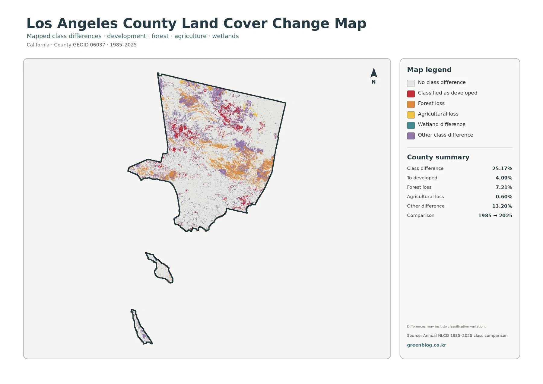
The map notes that differences may include classification variation. That warning should shape the entire interpretation. Use the change product to find areas where the two dates disagree, check the 2025 land-cover class at the same location, and then bring in additional imagery or local records if the cause matters.

Choosing the right map depends on whether the question is urban, ecological, or historical

For an urbanization discussion, the general map and impervious map are the strongest pair. Developed cover shows the broad metropolitan landscape, while impervious percentage shows how intensely roofs and pavement occupy that landscape. The southern mainland and northern Antelope Valley clusters are both visible, but their continuity and surrounding open land are very different.

For mountains and open space, the forest-and-farmland map is easier to read because the developed south is simplified. The Santa Monica Mountains, central and eastern mountain belts, northern shrubland, and forest patches can be compared without the detailed urban classes competing for attention. LA County’s General Plan and Conservation and Natural Resources Element provide policy context but should not be mistaken for land-cover data.

For long-term analysis, introduce the change map only after the current pattern is clear. A red or purple change cell does not tell the reader what covers that location today. Keeping a 2025 map beside the 1985–2025 comparison makes the result easier to interpret and reduces the risk of turning classification differences into unsupported causal claims.

Download the four original JPG maps

The WebP versions on this page are intended for quick viewing. The downloadable ZIP contains four original JPG maps: 2025 general land cover, forest and farmland, impervious surface and developed land, and the 1985–2025 land-cover change comparison. Because the maps use the same county boundary, they can be placed side by side in reports, presentations, lessons, or research notes.

Keep the legend and date visible when reusing the images. Shrubland, grassland, and forest are separate classes; developed cover is not the same as impervious percentage; and the change map compares two years. Removing those labels can make a correct map misleading.

These are county-scale reference graphics rather than parcel surveys or regulatory maps. They do not replace zoning, assessor records, legal wetland boundaries, site plans, or permits. LA County Planning’s General Plan and Z-NET are appropriate sources when the question is legal land use rather than physical surface cover.

Scale and classification limits matter more in a county this complex

Annual NLCD products generally use raster cells about 30 meters across. One cell can contain a roof, street, trees, lawn, and bare soil even though the land-cover map must assign a dominant class and the impervious product must summarize hard-surface fraction. This is especially important along Los Angeles County’s complicated urban-mountain boundaries.

Small reservoirs, narrow streams, wetland edges, hillside development, and thin transportation corridors can be generalized at this scale. The images are designed for broad county patterns, not for measuring a property line or a building footprint. A sharp-looking class boundary should therefore not be treated as a surveyed boundary on the ground.

The date is another limit. The current-condition maps represent 2025, so development, fire, vegetation recovery, or other surface changes after that year are not included. The change product compares only 1985 and 2025 and cannot reconstruct every event that occurred in between.

Land use and land cover also answer different questions. LA County Planning explains that land-use policy and zoning determine what types and intensities of uses are allowed on property. A red developed cell in the land-cover map says nothing by itself about zoning or future development rights, just as a shrubland cell does not identify ownership or conservation status.

Used with those limits in mind, the four-map set captures an unusually diverse county: an intensely built southern metropolis, separate northern settlement clusters, broad shrub-covered mountains and valleys, smaller forest and grassland areas, and offshore islands with very little hard surface. The maps are most useful when each layer is allowed to answer its own question rather than being forced into a single land-use interpretation.

Frequently Asked Questions

Sources and reference links

Land-cover and impervious-surface classifications can be reviewed through MRLC Annual NLCD Data and the USGS Annual NLCD Land Cover Classification. County boundary and FIPS reference data are available from U.S. Census Bureau TIGER/Line.

Local planning and natural-resource context can be checked through the Los Angeles County General Plan 2035, Conservation and Natural Resources Element, and Santa Monica Mountains North Area Plan. The LA County Planning Map Catalog includes area maps and a Santa Catalina Island Local Coastal Plan map.

Related Maps

• Alameda County California Land Cover Map
• Alpine County California Land Cover Map
• Amador County California Land Cover Map