Franklin County Alabama Land Cover Map presents a 2025 landscape where forest still covers more than half of the county, but the balance changes noticeably from west to east. Forest accounts for 54.78%, agriculture 24.55%, developed land 8.05%, shrubland 4.45%, and grassland 3.28%. The western half is more heavily wooded, while larger agricultural areas become much more common toward the eastern side. Several developed clusters interrupt that pattern rather than forming one continuous urban area.
Four matching map views are included on this page: general land cover, forest and farmland, fractional impervious surface, and mapped class differences between 1985 and 2025. The four original JPG maps are available in one download for reports, lessons, presentations, county comparisons, and printed reference. Each source JPG is 2480 × 1754 pixels, while the article previews use 1800 × 1273 WebP images. The maps describe surface cover; they do not replace parcel, zoning, survey, engineering, or permitting records.
Table of Contents
The clearest 2025 pattern is a wooded west and a more agricultural east
Dark-green forest occupies broad, connected areas across the western half of Franklin County and remains common through the center. The eastern side looks different. Yellow agricultural classes appear in much larger and more frequent patches there, especially near the northeastern and eastern edges. The transition is gradual rather than a straight dividing line: forest and farmland interlock across the middle, creating a mixed landscape instead of two isolated zones.
The 2025 summary confirms what the colors suggest. Forest is the dominant class at 54.78%, while agriculture reaches 24.55%. Together they describe most of the county, but their shapes matter as much as the totals. Forest tends to form larger continuous areas, while agriculture is broken into many fields and open patches. That distinction is useful when comparing Franklin County with a county that has a similar forest percentage but a different arrangement of farms and wooded land.
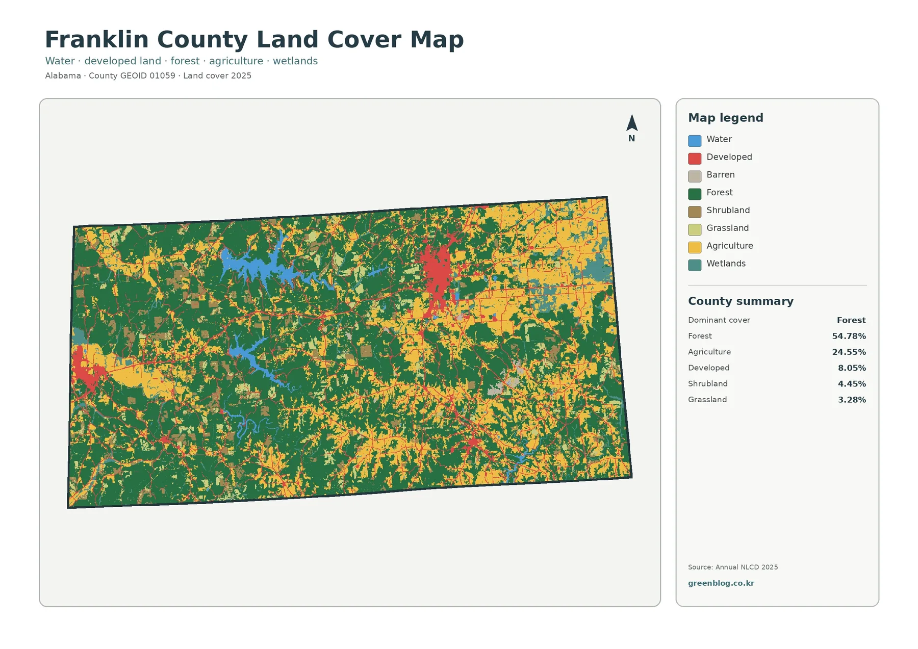
Developed land is 8.05% and is concentrated in several places. One of the largest red clusters appears in the north-central to northeastern portion of the county. Another strong concentration sits near the western edge, with smaller developed areas and narrow connecting traces elsewhere. The map therefore does not support a description of development as evenly spread. It is more accurate to say that built cover forms distinct centers linked by thinner developed corridors and scattered local patches.
Water and wetlands are present but occupy much smaller shares than forest or agriculture. In the forest-and-farmland summary, water accounts for 1.77% and wetlands for 2.80%. Blue water forms several branching shapes in the western and central portions, and another smaller water feature appears toward the southeast. Wetland colors occur in narrower patches around parts of the county. These classes help break up the forest-and-farm pattern, but they should not be treated as legal water or wetland boundaries.
The forest-and-farmland map separates fields, pasture, open land, and water more clearly
The second map reduces the visual weight of developed classes so that the rural cover is easier to compare. Forest remains 54.78% and agriculture totals 24.55%. Grassland is 3.28%, shrubland 4.45%, wetlands 2.80%, and water 1.77%. The legend also separates cropland from pasture or hay, allowing the agricultural share to be read as more than one type of open land.
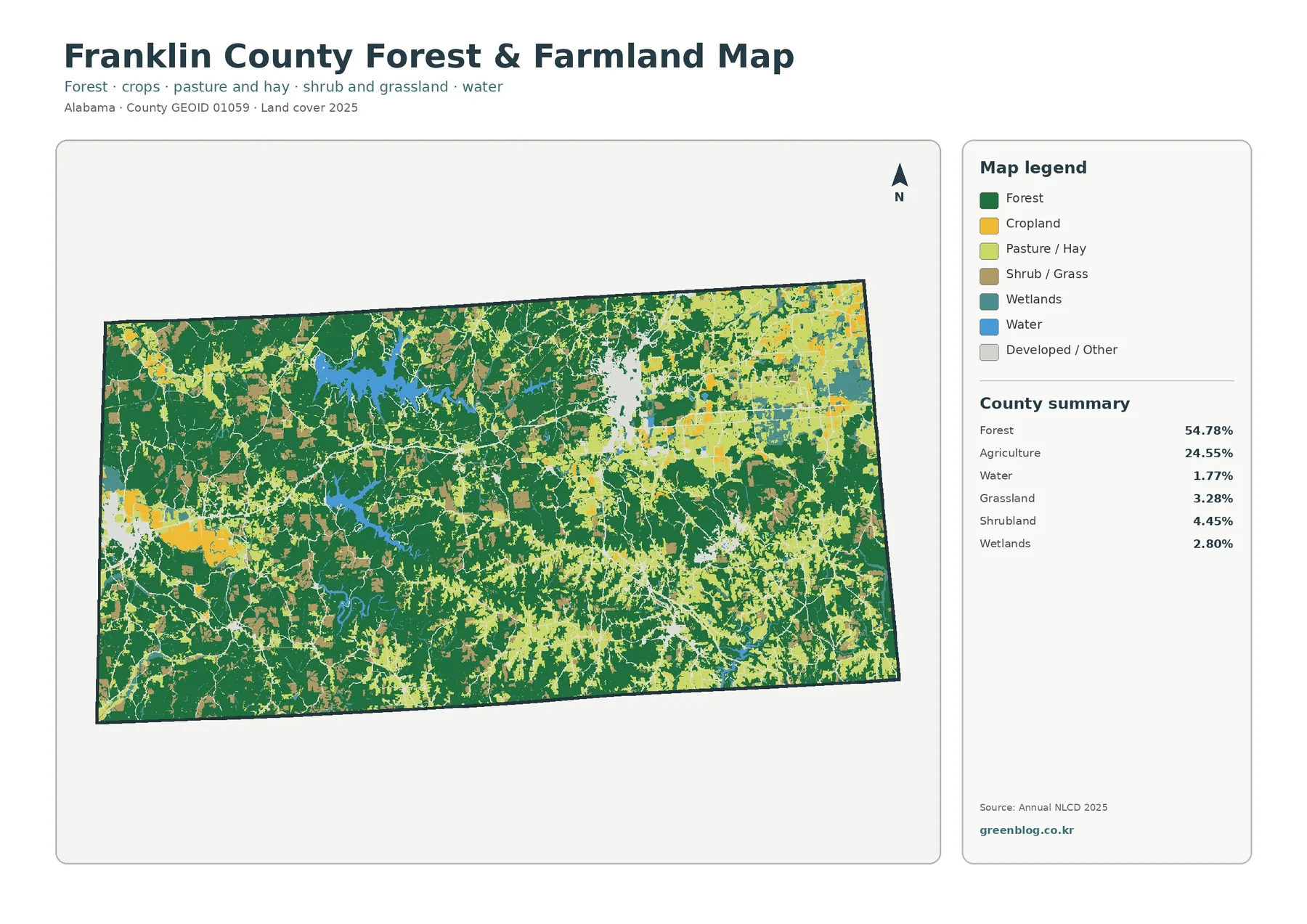
The western side contains large blocks of forest with agricultural openings scattered between them. Several blue water bodies also interrupt the wooded pattern there. Moving east, farm colors become more common and often occupy broader areas, although forest still threads between many fields. The southeastern portion returns to a more mixed arrangement, with forest, farms, open grass or shrub cover, and a smaller blue water feature all visible in the same general area.
This map is well suited to questions about landscape composition. A student can compare how continuous forest is in different parts of the county, identify where agriculture forms broad blocks, or examine where water breaks up woodland. It cannot identify a particular farm, crop owner, timber tract, conservation easement, or zoning district. A raster land-cover class describes the mapped surface condition at the dataset scale, not the legal status or ownership of a parcel.
The cropland and pasture colors are especially useful because two areas can both contribute to the 24.55% agriculture total while looking different on the map. Some open areas appear as compact field groups; others are narrow strips or smaller patches surrounded by forest. Keeping those forms separate is more informative than repeating a single countywide percentage. It also helps explain why agricultural land can be important even in a county where forest remains the majority cover.
Impervious surface is low countywide but clearly concentrated around developed centers
Fractional impervious surface measures the share of each mapped cell covered by hard materials such as pavement and rooftops. Franklin County has a mean impervious value of 1.54%, and 0.73% of the county is mapped at 50% or greater imperviousness. Developed cover is 8.05%, which is much larger because a developed land-cover cell can include lawns, trees, bare soil, and other permeable surfaces along with roads and buildings.
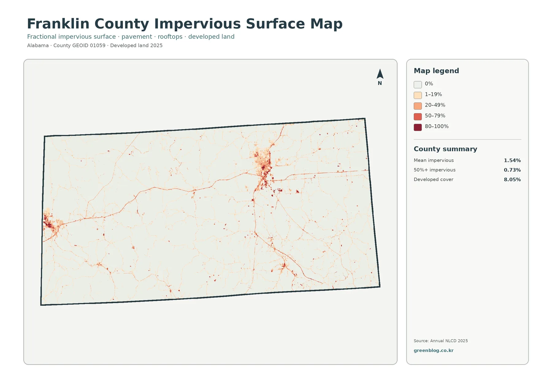
Most of the county is pale on this map, confirming that hard surfaces occupy a small share overall. The strongest dark concentration lies in the north-central to northeastern area, matching one of the large developed clusters visible on the general land-cover map. A second compact concentration appears near the western edge. Thin lines and smaller points extend away from those centers, while large forested and agricultural areas contain little mapped impervious surface.
The relationship between the two maps is useful because “developed” and “impervious” are not synonyms. The land-cover map answers where a cell is classified as developed. The impervious map asks how much of a cell is covered by hard surface. A low-density developed area can therefore appear red on the land-cover map but remain light on the impervious image. This distinction is important when comparing settlement intensity or discussing broad stormwater context.
The impervious image is not a drainage or infrastructure plan. It does not show culverts, storm pipes, channel direction, detention facilities, or property-scale runoff. Narrow roads and individual buildings can also be smaller than the display scale. Its strongest use is countywide comparison: it identifies where hard surfaces are concentrated and where the surrounding landscape remains mostly permeable.
Water is most visible in the wooded west and central portions
Although open water represents only 1.77% in the supplied forest-and-farmland summary, it has a strong visual presence because several blue shapes are large and branching. The most noticeable group lies in the western to west-central portion of the county, where water cuts through a heavily forested landscape. Additional blue features occur through the center and toward the southeast. Their shapes make them useful orientation points when comparing the four maps.
Wetlands account for 2.80%. They appear as narrower teal patches and small connected areas rather than dominating the county. The map supports describing where wetland cover is mapped in relation to forest, farmland, and water, but it does not identify jurisdictional wetlands. Regulatory wetland boundaries may depend on field evidence, soils, vegetation, hydrology, and agency procedures that are not represented by a countywide land-cover raster.
Water and wetlands also should not be merged into one percentage. Open water and wetland are separate classes with different meanings in the legend. Keeping them separate prevents a large reservoir-shaped feature from being described as wetland or a wetland corridor from being described as open water. For watershed education, the two categories can be compared visually before a reader moves to a dedicated hydrography map for named streams, lake boundaries, or drainage networks.
The 1985–2025 map marks class differences without assigning a cause
The change product compares the mapped class at two endpoints, 1985 and 2025. The supplied summary reports a class difference across 30.55% of Franklin County. Within the listed categories, 1.77% is classified as “to developed,” 9.03% as forest loss, 3.41% as agricultural loss, and 15.97% as other class difference. A wetland-difference class is included in the legend, but no separate countywide percentage is printed for it.
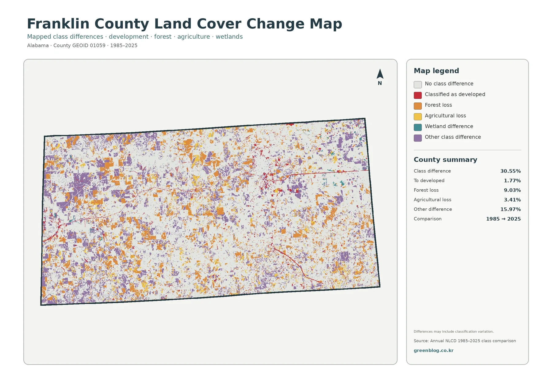
Orange forest-loss and purple other-difference cells occur widely across the county. They are especially noticeable in the western half, but they also appear through the center and east. Red “to developed” cells form much smaller concentrations, with clusters around existing developed areas and along several narrow lines. Yellow agricultural-loss cells are scattered in smaller patches. The distribution makes the change map useful for locating areas that deserve closer investigation.
The map itself provides an important warning: differences may include classification variation. A cell that receives a different class in 1985 and 2025 was not necessarily physically transformed in a simple one-step process. Mixed pixels, seasonal vegetation, imagery quality, sensor differences, or changes in classification methods can affect the assigned label. Some highlighted areas may reflect real clearing, regrowth, farming changes, or construction, but this two-date comparison cannot prove the cause.
For historical research, use the map as a screening layer rather than a final timeline. Areas with many highlighted cells can be checked against intermediate Annual NLCD years, historical aerial photographs, or other dated records. A location may have changed more than once between 1985 and 2025, and a two-endpoint map cannot show every intermediate condition. Conversely, a location that returned to its original class may appear unchanged even if its history was more complicated.
Reading the four maps in sequence keeps unlike measurements separate
A practical sequence begins with the general 2025 land-cover map to establish the countywide mix. The forest-and-farmland view then clarifies how woodland, cropland, pasture, shrub or grass cover, wetlands, and water are arranged. The impervious map focuses on hard-surface intensity inside the broader developed pattern. The final change map identifies where endpoint classifications differ between 1985 and 2025.
The numerical summaries should stay tied to those definitions. Developed land is 8.05% in 2025, but only 1.77% is listed as “to developed” in the endpoint comparison. Mean imperviousness is 1.54%, a third measurement that describes hard-surface fraction rather than a land-cover class. Forest is 54.78% today, while 9.03% is highlighted as forest loss between the endpoints. These values should not be added or subtracted to create one development or forest-change rate.
The same rule applies when Franklin County is compared with another county. Match 2025 forest to 2025 forest, mean imperviousness to mean imperviousness, and the 1985–2025 class-difference product to an equivalent comparison. This keeps a classroom exercise, regional report, or presentation understandable because each visual and percentage is being compared with the same kind of measure.
The JPG set works well for county reference, lessons, and presentations
The downloadable ZIP contains the four original Franklin County JPG maps using the same county extent. A report can begin with the general 2025 map, move to the forest-and-farm distribution, focus on developed hard surfaces, and finish with the 1985–2025 comparison. The consistent boundary makes the images easy to place side by side without changing orientation between topics.
Each source JPG is 2480 × 1754 pixels. The package identifies that as the original source resolution and does not mark the files as meeting a higher A3 reference standard. If a map will be printed at a large size, test the legend and small text at the intended dimensions. Enlarging a raster image can make pixels larger, but it cannot create new geographic detail that was not present in the source.
Scale, observation year, and legal purpose set clear limits
Annual NLCD land cover is raster data. In simple terms, the landscape is divided into grid cells and each cell receives a representative class. At roughly 30-meter land-cover resolution, a small road, field edge, stream margin, building group, or patch of trees can share a cell with another surface. A sharp color boundary in the JPG therefore should not be treated as a surveyed property line.
The current-cover maps represent 2025 in the supplied package. Conditions after that year are outside the image. The change product compares only 1985 and 2025 endpoints, so it cannot identify the exact year a change occurred or every intermediate step. Recent development, forestry activity, field conversion, or vegetation recovery should be checked with newer imagery or other current sources when timing matters.
Land cover is also different from legal land use. A cell mapped as agriculture does not establish agricultural zoning, ownership, tax treatment, or crop type. Forest does not identify timber rights or protected status. Developed cover does not establish a building right, and wetland cover is not a jurisdictional determination. These maps are strongest for countywide description and preliminary comparison; site-level decisions require the appropriate current parcel, regulatory, survey, engineering, or field records.
Frequently Asked Questions
What is the largest land-cover class in Franklin County?
Forest is the largest class in the supplied 2025 summary at 54.78%. Agriculture follows at 24.55%, developed land at 8.05%, shrubland at 4.45%, and grassland at 3.28%. The distribution is not uniform: the west is more heavily forested, while larger agricultural patches are more common toward the east.
Why is developed cover 8.05% while mean imperviousness is only 1.54%?
They measure different things. Developed land is a categorical land-cover class and can include lawns, trees, soil, and other permeable surfaces. Imperviousness measures the fraction of hard surface such as pavement and rooftops. Franklin County’s mean impervious value is 1.54%, and 0.73% of the county is at least 50% impervious.
Does 30.55% class difference mean that 30.55% of the county was physically transformed?
No. It means that 30.55% of mapped cells received different classes in the 1985 and 2025 endpoint comparison. The map explicitly warns that classification variation may be included. Some differences may represent real land-cover change, while others can reflect mixed pixels, imagery conditions, or classification differences.
Map File Information
The ZIP contains four original Franklin County JPG maps: 2025 land cover, forest and farmland, impervious surface, and mapped land-cover class differences from 1985 to 2025.
- File Type: ZIP containing four JPG images
Related Maps
- Autauga County Alabama Land Cover Map
- Baldwin County Alabama Land Cover Map
- Barbour County Alabama Land Cover Map
Sources and data notes
- MRLC Annual NLCD Data — official access point for Annual NLCD land-cover and developed-surface products.
- USGS Annual NLCD Land Cover Classification — official descriptions of the mapped land-cover classes.
- U.S. Census Bureau TIGER/Line Shapefiles — official geographic boundary reference.
Green Map creates custom-edited map images using open geographic data sources such as geoBoundaries, Natural Earth, OpenStreetMap, and government open data.
These maps are edited visual materials, not raw data files, and are provided for education, documents, presentations, and graphic reference.