The 2025 EIA data compare fuel consumption for electricity generation and useful thermal output across all 50 states plus Washington, D.C. The series is restricted to the EIA fuel category “natural gas & other gases,” the annual total-consumption-btu field, and a common unit of million MMBtu. It should not be read as total household gas use, total state natural gas demand, or natural gas production. The scope is narrower: fuel input used for electricity generation and useful thermal output in the selected operational-data series.
Adding the 51 jurisdiction rows produces 15,342.437 million MMBtu. Texas is highest at 2,652.885, followed by Florida at 1,466.630 and Pennsylvania at 1,089.012. Those three account for 33.9% of the row sum, while the top ten account for 60.3%. The mean is 300.832, considerably above the median of 162.589, which signals a strongly right-skewed distribution in which a limited number of very large state values pull up the average.
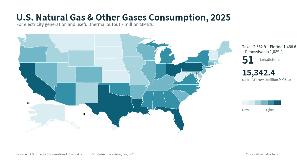
Table of Contents
What this EIA measure actually covers
The full metric describes consumption of fuels for electricity generation and useful thermal output in BTU terms. That distinction matters because fuel input is not the same thing as electricity output. Plants can have different conversion efficiencies, operating hours, combined heat-and-power configurations, and mixes of electric and thermal output. A state can therefore have a large fuel-input figure without an identical ranking in electricity generation. The data are best used to compare the scale of fuel input under one consistent EIA definition.
The fuel facet is fixed to the EIA category “natural gas & other gases.” The underlying package does not provide a separate breakout for every component inside that category, so the analysis keeps the official label intact rather than treating every unit as natural gas alone. Likewise, the sector facet and field are kept fixed across all rows. This controlled scope is what makes a state-by-state comparison meaningful; mixing other fuel categories or a different EIA field would change the statistical identity of the series.
States with the largest 2025 values
Texas stands apart from the rest of the distribution. Its 2,652.885 million MMBtu is about 1.81 times Florida’s 1,466.630. Pennsylvania is third at 1,089.012, followed by Louisiana at 751.757, Ohio at 632.858, and California at 629.457. New York, Alabama, Virginia, and Michigan complete the top ten. These are absolute quantities, not values normalized for population, state GDP, generation, or installed capacity. Large power systems and states with substantial gas-fired or thermal-output activity will naturally tend to rank higher on an absolute measure.
| Rank | State | 2025 value (million MMBtu) |
|---|---|---|
| 1 | Texas | 2,652.885 |
| 2 | Florida | 1,466.630 |
| 3 | Pennsylvania | 1,089.012 |
| 4 | Louisiana | 751.757 |
| 5 | Ohio | 632.858 |
| 6 | California | 629.457 |
| 7 | New York | 551.249 |
| 8 | Alabama | 528.622 |
| 9 | Virginia | 486.584 |
| 10 | Michigan | 460.362 |
Concentration is substantial. Texas alone represents 17.3% of the 51-row sum. The top three account for 33.9%, the top five 43.0%, and the top ten 60.3%. These shares are derived from the supplied state and D.C. rows; they are not copied from a separate EIA national-total series. That distinction is useful because an official national aggregate can have its own accounting scope or revisions. For reproducible state comparisons, the safest denominator is the same set of rows used in the analysis.
Why the median is more informative than the mean
The mean across the 51 jurisdictions is 300.832 million MMBtu, but the median is only 162.589. The median corresponds to Kentucky when the values are ordered. The first quartile is 56.739 and the third quartile is 425.090, so half of the jurisdictions fall roughly between those two values. The mean is about 1.85 times the median because very large observations—especially Texas, Florida, and Pennsylvania—pull the arithmetic average upward.
That skew affects how the map should be read. A single average is not a good description of a typical jurisdiction in a distribution with a long upper tail. The map therefore uses value bands to preserve visual separation among low and mid-range states while still showing the very large values. Exact numbers should be read from the data table rather than inferred from color alone. The map answers a spatial question—where the larger and smaller observations are located—not an efficiency or per-capita question.
Low values and the special case of zero
Hawaii is recorded at 0.000 million MMBtu. This is an observed zero in the source data, not a missing value that has been replaced with zero. Vermont is next at 0.088, followed by Washington, D.C. at 1.334. Montana, Nebraska, South Dakota, Alaska, North Dakota, West Virginia, and New Hampshire are also near the bottom. A low value does not mean a state has no electricity generation or no natural gas use in general. It only means the selected EIA fuel category is small within this specific electricity-generation and useful-thermal-output measure.
| Rank from low | State or district | 2025 value (million MMBtu) |
|---|---|---|
| 1 | Hawaii | 0.000 |
| 2 | Vermont | 0.088 |
| 3 | District of Columbia | 1.334 |
| 4 | Montana | 13.480 |
| 5 | Nebraska | 19.839 |
| 6 | South Dakota | 23.092 |
| 7 | Alaska | 25.710 |
| 8 | North Dakota | 32.873 |
| 9 | West Virginia | 38.085 |
| 10 | New Hampshire | 40.381 |
Absolute quantities are especially sensitive to system size. A geographically small jurisdiction such as Washington, D.C. can be expected to look small in a state-level fuel-input ranking because its generation asset base is limited. Conversely, a state with a relatively small population can rank higher if it hosts substantial generation or combined heat-and-power facilities. This is why the ranking should not be converted into a judgment about household energy use, economic performance, or energy affordability. Those questions require different denominators and additional data.
The geographic pattern is broad, not confined to one region
Many high values occur in southern states—Texas, Florida, Louisiana, Alabama, Virginia, North Carolina, Georgia, and Mississippi all appear relatively high. Yet the upper part of the distribution also includes Pennsylvania, Ohio, New York, and Michigan, while California and Arizona stand out in the West. The pattern is therefore better understood as a feature of several large electricity systems that use substantial amounts of the selected gas category rather than as a single-region phenomenon.
The CSV does not identify the causal mechanism behind each state value. Fuel mix, generating capacity, plant utilization, combined heat-and-power activity, weather-driven demand, outages, and interstate electricity trade can all matter. The map shows where fuel input is large; it does not prove why it is large. A causal explanation would require additional EIA series such as generation by fuel, capacity, plant-level operations, or heat-output measures matched to the same period and geography.
What it means that the top ten exceed 60%
The top ten jurisdictions sum to 9,249.416 million MMBtu, or 60.3% of the 51-row total. That degree of concentration means a relatively small group of states shapes the national state-level distribution. It also explains why changes in a few large states could move the aggregate substantially from one year to the next. Still, this is concentration in fuel input, not market share in electricity sales, natural gas production, utility revenue, or generation ownership.
The map and ranking table complement each other. The map makes the spatial clustering visible, while the table shows that apparently similar color bands can hide substantial numerical gaps. Texas and Florida, for example, are both high but are separated by more than 1,186 million MMBtu. At the low end, several jurisdictions share the same broad visual band even though their operational circumstances may be very different.
How to compare 2025 with another year
This dataset is a single-year cross-section. Fuel consumption can change with gas prices, weather, plant retirements and additions, maintenance schedules, renewable output, coal and nuclear utilization, and electricity demand. A one-year rank should therefore not be treated as a permanent structural ranking. A trend analysis should retrieve multiple years from the same EIA route while holding the field, fuel facet, sector facet, unit, and geography constant.
Revision timing matters as well. Official energy datasets can be updated after an initial release. Re-querying 2025 at a later date may produce revised values for some states. For reproducibility, it is useful to retain the collection date, exact endpoint identity, and the state-level observations used in the article. The current package contains one complete observation for every state and D.C.; no missing value was imputed or replaced with a prior-year figure.
What this metric can and cannot tell you
The series can identify where the selected gas fuel category is used most heavily for electricity generation and useful thermal output, how unequal the state distribution is, and how concentrated the total is among the largest observations. It cannot directly measure generation efficiency, carbon emissions, wholesale or retail electricity prices, natural gas production, pipeline constraints, household gas demand, or the technology of individual plants. A high fuel-input value can coexist with very different output and efficiency profiles.
That makes the indicator a useful starting point rather than a complete energy-system scorecard. After locating the largest fuel-input states, analysts can combine the series with electricity generation to study input-output relationships, with capacity to examine utilization, or with emissions to explore environmental intensity. Those additions should be made explicitly because each changes the question being answered.
The most useful numbers to retain from the 2025 comparison
Texas leads at 2,652.885 million MMBtu, Florida is second at 1,466.630, and Pennsylvania is third at 1,089.012. The 51-row sum is 15,342.437; the median is 162.589; and the top ten make up 60.3% of that row sum. Hawaii’s 0.000 is a genuine reported zero, and none of the 51 jurisdictions is missing from the supplied 2025 table. Those facts provide a compact framework for interpreting the map without turning it into a broader claim than the source supports.
Use the table for exact values and the map for spatial context. When comparing this article with another EIA state series, check the route, field, fuel type, sector, year, and unit before drawing conclusions. Titles can sound similar even when one facet has changed, and that difference can produce a genuinely different metric.
Frequently Asked Questions
Does this measure total natural gas consumption in each state?
No. It is the EIA fuel-consumption series for electricity generation and useful thermal output, restricted to the natural gas & other gases category. It does not represent all residential, commercial, industrial, or pipeline gas use.
Is Hawaii’s zero a missing value?
No. Hawaii is reported as 0.000 million MMBtu in the supplied 2025 observations. All 50 states and Washington, D.C. have a value; no missing observation was replaced with zero.
Can this dataset explain why Texas is highest?
Not by itself. The table measures fuel input, not the causes behind it. Explaining Texas would require additional data on generation, capacity, utilization, fuel mix, combined heat and power, and other operating factors.
Related Articles
Green Map creates custom-edited map images using open geographic data sources such as geoBoundaries, Natural Earth, OpenStreetMap, and government open data. These maps are edited visual materials, not raw data files, and are provided for education, documents, presentations, and graphic reference.