Forest is the defining 2025 surface pattern in Talbot County, covering 68.98% of the mapped area. Grassland accounts for 7.48%, shrubland 6.60%, agriculture 6.10%, and developed cover 4.67%. The map is not a single unbroken green block, however. Open land breaks the forest into many pockets, while developed cover appears mainly as small clusters and thin lines rather than a broad urban field.
Four views are provided here: current land cover, forest and farmland, impervious/developed land, and a 1985–2025 class-difference map. The article uses WebP previews, while the four original JPG maps are available together in one ZIP. Reading the views side by side makes it easier to separate forest dominance from open rural cover, and to distinguish mapped development from the much smaller fraction of hard, impervious surface.
Table of Contents
A 68.98% forest share dominates the county, but the open-land pattern is far from uniform
The supplied county summary places forest far ahead of every other 2025 class. Grassland is 7.48%, shrubland 6.60%, agriculture 6.10%, and developed land 4.67%. The forest-and-farmland panel separately reports wetlands at 4.45% and open water at 0.84%. Barren land appears in the legend, but the package does not provide a separate barren percentage in the summary, so no residual value has been calculated or assigned to it.
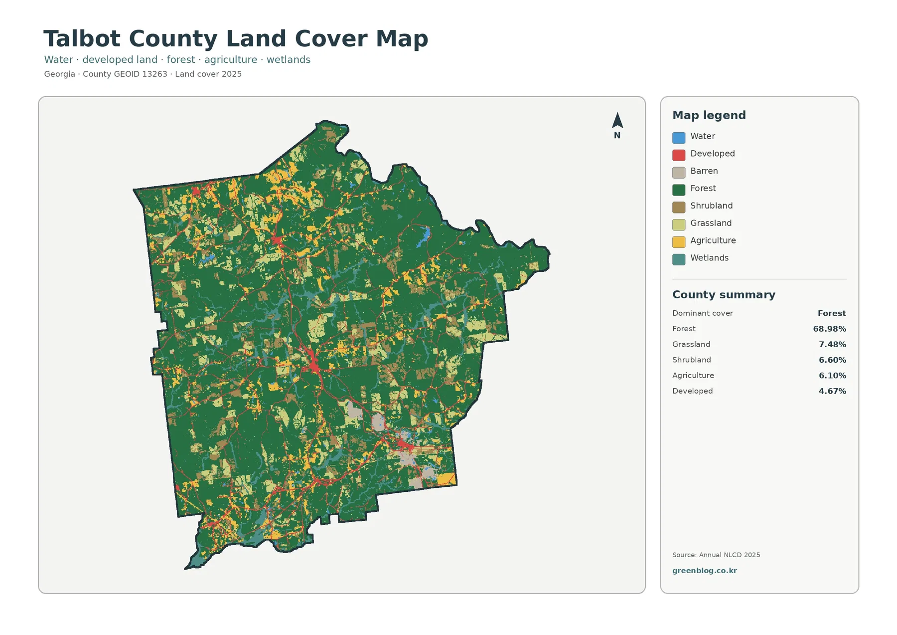
Dark green extends across most of the county outline. Larger groups of light green, brown, and yellow are more noticeable in parts of the west and northwest, with additional open patches scattered through the southern and central areas. The east and northeast contain broader runs of forest in the supplied image. These are county-scale patterns, not parcel boundaries, but they make clear that the nonforest classes are clustered rather than evenly sprinkled everywhere.
Developed cover has a different geometry. Instead of filling a large metropolitan footprint, it forms several compact concentrations linked by narrow linear traces. The map does not label streets or towns, so a colored line should not be assigned to a particular highway from this image alone. It is safer to describe the visible pattern as small settlement concentrations and developed corridors within a predominantly forested county.
Water and wetlands also need to be kept separate. Open water is 0.84% in the supplied summary, while wetlands account for 4.45%. Blue cells represent surface water; teal wetland cells represent a different land-cover class associated with wet conditions and wetland vegetation. Neither class is a legal wetland determination, flood zone, ownership boundary, or water-access map.
| 2025 map summary | Share |
|---|---|
| Forest | 68.98% |
| Grassland | 7.48% |
| Shrubland | 6.60% |
| Agriculture | 6.10% |
| Developed | 4.67% |
| Wetlands | 4.45% |
| Water | 0.84% |
These values describe what covers the ground, not how land is zoned or who owns it. A forest-classified cell may be private, public, residentially zoned, or part of a larger tract with another legal use. Likewise, an agriculture-classified cell does not establish a farm parcel or agricultural zoning. Parcel, zoning, permitting, and ownership questions require records created for those purposes.
Only 0.82% mean impervious cover separates the small built nodes from the forest background
Impervious surface means pavement, rooftops, parking areas, and other hard surfaces that keep water from soaking directly into soil. The supplied map divides each raster cell into 0%, 1–19%, 20–49%, 50–79%, and 80–100% impervious categories. Talbot County has a mean impervious value of 0.82%, and only 0.16% of the county is in cells above 50% impervious. Those figures are much smaller than the 4.67% developed-cover share because the two layers measure different things.
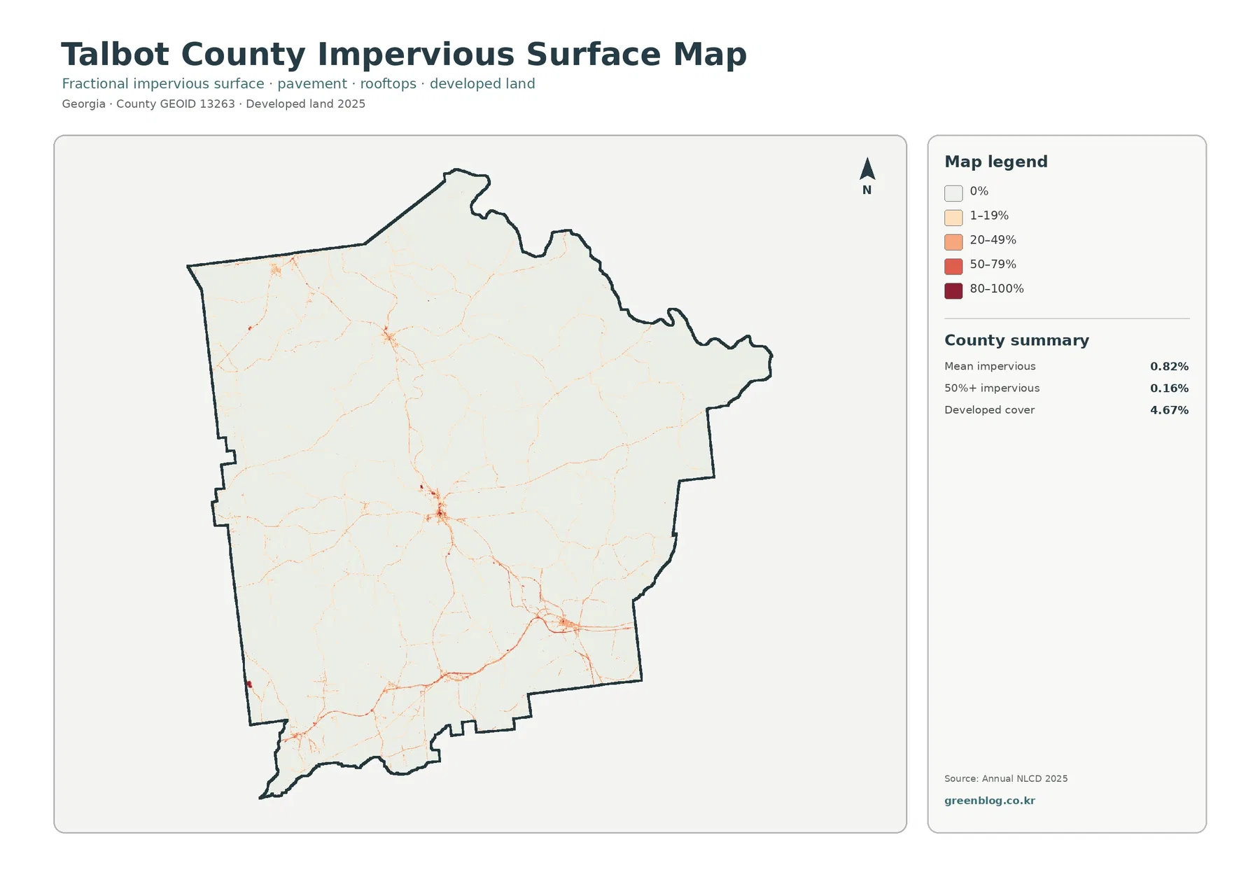
Most of the county is almost white on the impervious view. Darker orange and red appear in a few small centers, with pale lines extending outward. The strongest clusters do not merge into a large continuous urban area. At county scale, the pattern is better described as a set of small built locations connected through a rural road network than as a single developed core.
Talbot County Public Works provides useful context for those thin lines. Its road page lists 250 miles of registered paved roads and 212 miles of registered unpaved roads. That does not tell us which line in the impervious map is which road, but it does explain why a complete road network should not be reconstructed from hard-surface color alone. Unpaved roads and low-width surfaces may look very different from major paved routes in a 30-meter raster product.
The gap between 4.67% developed land and 0.82% mean impervious surface is also expected in low-density places. A developed raster cell can contain a house, lawn, trees, bare soil, and a driveway. The impervious layer estimates the hard-surface fraction inside the cell rather than treating the whole cell as pavement. A small town can therefore have recognizable developed cover without producing a large block of high impervious values.
This map is useful for finding relative concentrations of hard surface, but it is not a drainage or flood-risk model. Runoff also depends on slope, soils, storm intensity, channels, culverts, and surrounding land cover. For engineering or hazard work, the impervious layer should be combined with elevation, hydrology, soil, and local infrastructure data.
Forest, grassland, shrubland, and agriculture form a mixed rural cover rather than one simple farm belt
The forest-and-farmland view strips away some of the visual competition from developed land and makes the rural classes easier to compare. Forest remains dominant at 68.98%, but agriculture is only one part of the open-land story. Grassland at 7.48% and shrubland at 6.60% are each slightly larger than agriculture at 6.10%. Wetlands and water remain visible as separate classes, which helps prevent every nonforest patch from being interpreted as farmland.
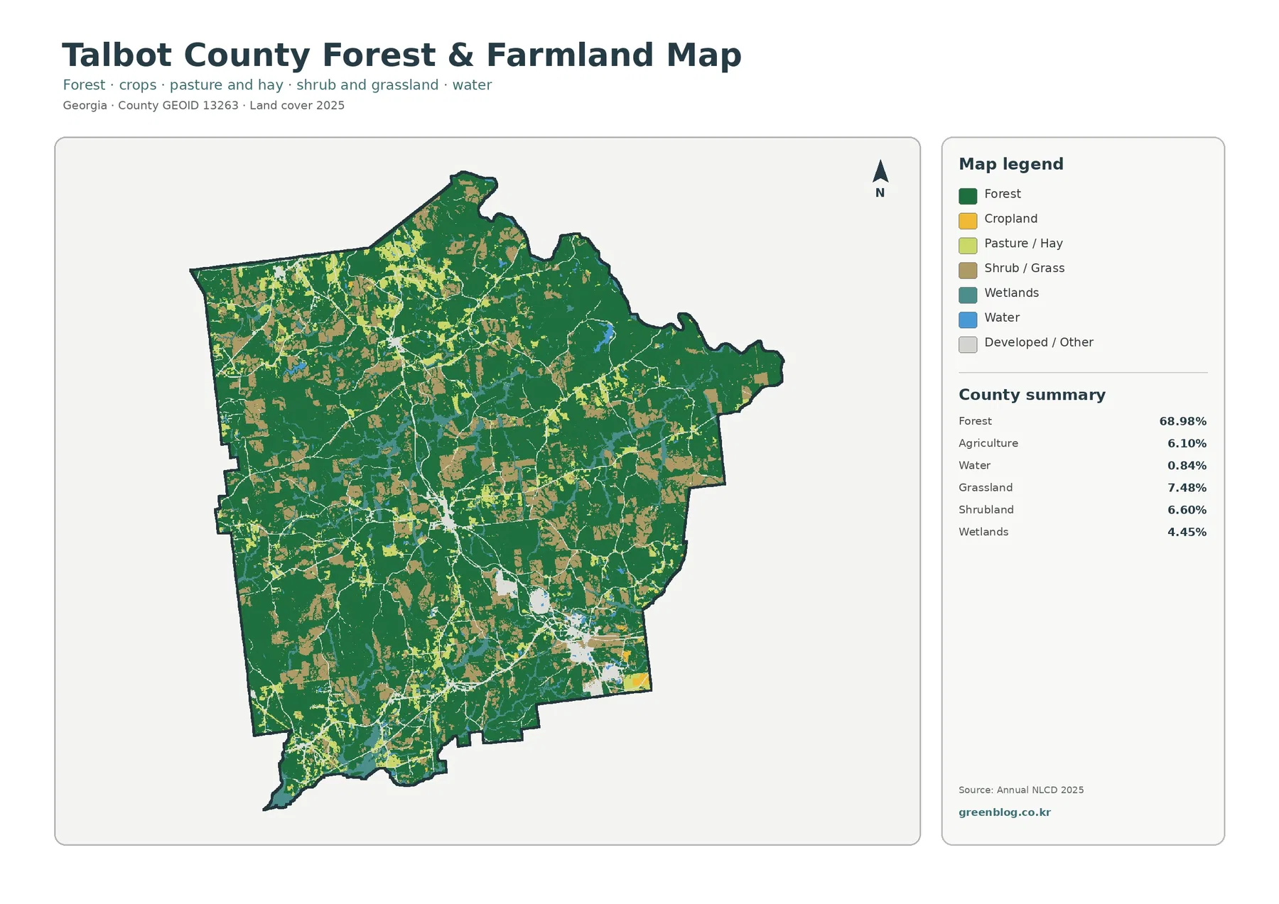
Many of the larger open patches occur in the western and northwestern portions of the map, while smaller groups are spread through the center and south. Forest blocks are broader in much of the eastern side. The boundaries between these classes are irregular and frequently interlocked, so the landscape is better understood as a forest-heavy mosaic than as a clean east-west split between farms and woods.
Agriculture-colored cells identify mapped cropland, but the image cannot tell the reader what crop is being grown, whether a field is currently active, how many farms operate nearby, or whether a neighboring grassland cell is pasture, hay, or another open cover. Those questions need agricultural statistics or local records. The purpose of this view is narrower: it shows where major rural surface classes occur relative to the dominant forest.
The University of Georgia Extension office for Talbot County currently provides Agriculture & Natural Resources programming. That county-specific resource is a useful next step when a reader needs practical local information about agriculture, forestry, soils, or related topics. It should not be treated as an explanation for the mapped percentages; the land-cover image and the Extension program describe different kinds of information.
Scale matters along every field edge. Annual NLCD products generalize the landscape at roughly 30-meter resolution, so a cell can mix trees, grass, a narrow road, and part of a field. Fine hedgerows, small clearings, and individual property lines can be simplified or absorbed into a neighboring class. The map is strong for county-wide comparison but too generalized for surveying or parcel-level decisions.
The 41.15% 1985–2025 class difference is mostly not a developed-land change
The change map compares the class assigned in 1985 with the class assigned in 2025. The supplied summary reports a total class difference of 41.15%. Within that total, 0.88% is categorized as changing to developed, 13.13% as forest loss, 2.29% as agricultural loss, and 24.68% as other class difference. Wetland difference is also shown in the legend, but its percentage is not separately printed in the summary.
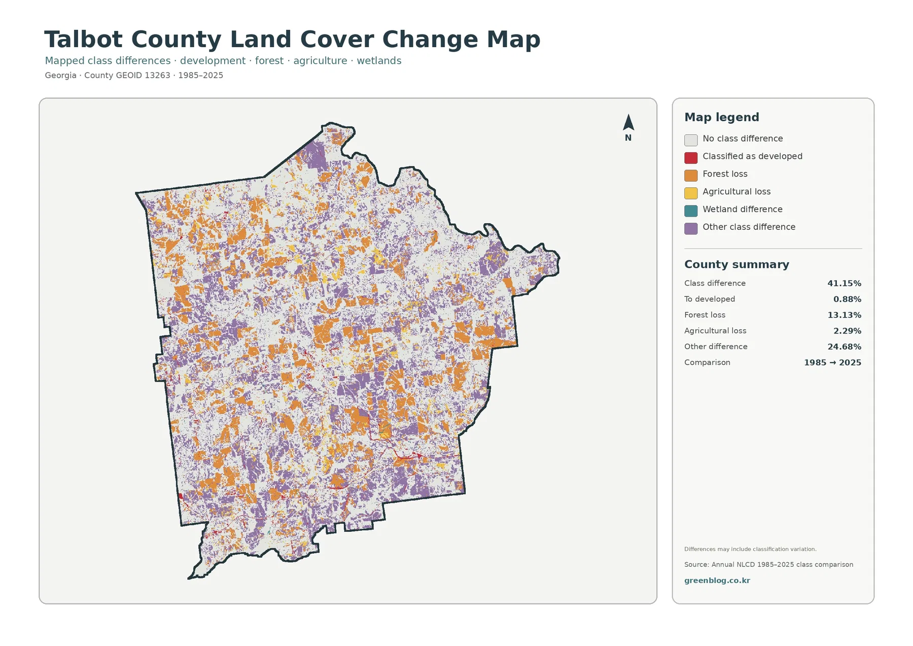
Orange forest-loss patches and purple other-difference patches are distributed widely across the county. White no-difference areas remain substantial, while red change-to-developed cells occupy a much smaller footprint and tend to appear near present developed traces. The visual balance matches the summary: the map records a broad set of classification changes, not a county that became 41.15% urban.
The 13.13% forest-loss category also should not be described as verified permanent deforestation without additional evidence. A two-date land-cover comparison can reflect real clearing, harvest, conversion, regrowth cycles, different vegetation states, image conditions, cell boundaries, and classification variation. The map itself includes a note that differences may include classification variation. Historical aerial photographs and intermediate-year data are needed to establish what happened at a specific site.
The largest printed component is the 24.68% other class difference. By definition, that value combines changes that are not summarized as developed, forest loss, or agricultural loss. It should not be given a single cause. Similarly, 2.29% agricultural loss does not mean farm output or the number of farms fell by 2.29%; it means the endpoint land-cover class differs from agriculture for those mapped cells.
Because this is an endpoint comparison, it does not identify the year when a change occurred. A cell that changed in the late 1980s and a cell that changed shortly before 2025 may appear the same. The layer is best used to locate areas for follow-up, then paired with more dates, aerial imagery, forestry records, or planning documents if timing and cause matter.
Talbotton and Big Lazer Creek add local context without turning unlabeled pixels into named places
Talbot County government identifies Talbotton as the county seat and notes that Big Lazer Creek Wildlife Management Area is in the county. The county also describes a 196-acre public fishing lake at that facility, which is operated by the Georgia Department of Natural Resources. These facts provide real local reference points for a map that otherwise contains no place-name labels.
They also illustrate why a base map is sometimes necessary. A blue patch in the land-cover map should not automatically be labeled as the Big Lazer Creek public fishing lake, and a red impervious cluster should not be named Talbotton from color alone. To match a land-cover feature with a community, road, lake, or management area, compare the image with an official road, facility, or boundary map.
Georgia Department of Community Affairs planning pages list Geneva, Junction City, Talbotton, and Woodland in the Talbot County comprehensive-planning set. That is consistent with a county containing several small communities rather than one large continuous city. Still, the land-cover package does not label each community, so this article uses those names as regional context instead of claiming that a particular colored cluster belongs to a specific municipality.
The same caution applies to public land. The existence of Big Lazer Creek WMA does not mean every forest or wetland cell on the map is protected or publicly owned. Land-cover classes describe surface appearance, while management-area boundaries describe jurisdiction and access. Anyone planning recreation, hunting, fishing, or site access should use the current Georgia DNR maps and rules for that purpose.
Choose the view by the question, then keep the legend and year visible
Use the general land-cover map for the broadest county portrait. It places forest, developed land, agriculture, grassland, shrubland, wetlands, water, and other mapped classes in one frame. It is the best starting point for explaining why Talbot County reads as forest-dominant even though open rural patches and settlement traces are present throughout the outline.
Use the impervious view when the question is about hard surfaces rather than the broader developed class. The 0.82% mean value and 0.16% share above 50% impervious make the county-scale sparsity easy to communicate. Pairing it with general land cover is especially useful because it prevents readers from assuming that every developed cell is mostly pavement or rooftop.
For rural land-cover comparison, the forest-and-farmland image is more informative. It keeps grassland and shrubland distinct from agriculture, so the reader can see that open land is not synonymous with cropland. The change layer should come after the current maps because its colors describe differences between 1985 and 2025, not present-day land-cover classes.
When using the files in slides or reports, preserve the legend and summary panel. Cropping them out can turn a correct image into an ambiguous one, especially when similar colors have different meanings on the current and change maps. Captions should state “2025 land cover” for the current views and “1985–2025 class difference” for the change map.
Four 2480×1754 JPG maps are packaged together for download
The article previews are 1800-pixel WebP images intended for the web page. The downloadable archive contains four original JPG files at 2480×1754 pixels each: general land cover, forest and farmland, impervious/developed land, and the 1985–2025 land-cover change map. Their consistent county outline, legend placement, and summary area make them easy to compare side by side in a document or presentation.
The asset manifest does not mark these images as meeting an A3 high-resolution reference. They work well for screen use, ordinary documents, and many presentation layouts, but very large printing should be tested first. Thin impervious lines, small wetland branches, and legend text may soften when enlarged beyond the native pixel dimensions.
For a two-map layout, general land cover beside impervious surface gives a strong forest-versus-built comparison. Forest and farmland beside the change map works better when the subject is rural cover and long-term classification differences. If all four are used, leave enough space for the legends to remain readable rather than shrinking the maps until the classes can no longer be distinguished.
Resolution, observation dates, and legal definitions limit what the maps can answer
Annual NLCD mapping generalizes the surface into raster cells at roughly 30-meter scale. A single cell may contain trees, grass, a house, and part of a road. The assigned class or impervious percentage summarizes that cell rather than tracing every object. This is appropriate for county-level pattern analysis, but it cannot replace parcel surveys or detailed engineering data.
The current maps represent 2025 conditions in the supplied dataset. Construction, clearing, regrowth, or farming changes after that observation period are not included. The change map uses 1985 and 2025 as endpoints and does not provide a year-by-year history. Projects that depend on current site conditions should add recent aerial imagery, local records, and field verification.
Mapped wetlands and water are surface classifications, not regulatory determinations. They do not define FEMA flood zones, legal wetland boundaries, navigable waters, or public access. Likewise, forest cover does not establish a conservation easement or public ownership, and developed cover does not establish zoning or building rights.
The change layer identifies class differences, not causes. A developed-change cell near a road does not prove that the road caused the change, and a forest-loss cell does not reveal whether the process was harvest, conversion, storm damage, or classification variation. Cause requires a timeline and independent evidence.
The most reliable use is therefore descriptive: compare where the supplied classes are concentrated, where they transition, and how the 1985 and 2025 endpoints differ. When the question moves to ownership, regulation, flood risk, road status, development approval, or land-management history, move to the official dataset designed for that question.
Frequently Asked Questions
What is the dominant 2025 land-cover class in Talbot County?
Forest is the dominant supplied class at 68.98%. Grassland is 7.48%, shrubland 6.60%, agriculture 6.10%, and developed cover 4.67%. Wetlands and water are separately reported at 4.45% and 0.84% in the forest-and-farmland summary.
Why is developed cover 4.67% while mean impervious surface is only 0.82%?
A developed raster cell can still contain lawns, trees, bare soil, and other permeable surfaces. The impervious layer estimates the hard-surface fraction from pavement and rooftops, so a low-density developed area can count as developed while remaining only lightly impervious.
Does the 41.15% 1985–2025 class difference mean 41.15% of Talbot County became developed?
No. Only 0.88% is summarized as changing to developed. The map also reports 13.13% forest loss, 2.29% agricultural loss, 24.68% other class difference, and a mapped wetland-difference category, with a warning that classification variation may be included.
Map File Information
Download the four original Talbot County land-cover JPG maps in one ZIP: general land cover, forest and farmland, impervious/developed land, and 1985–2025 land-cover change.
- Printable Size: 2480×1754 pixels each
Related Maps
- Appling County Georgia Land Cover Map
- Atkinson County Georgia Land Cover Map
- Bacon County Georgia Land Cover Map
Sources and references
- MRLC Annual NLCD Data – Official access point for Annual NLCD land-cover and related products used for the supplied 2025 mapping.
- USGS Annual NLCD Land Cover Classification – Official explanation of Annual NLCD classes such as forest, developed land, agriculture, and wetlands.
- Talbot County, Georgia – About Talbot County – Official county information about Talbotton, Big Lazer Creek Wildlife Management Area, and the public fishing lake.
- Talbot County Public Works – Roads – Official county information on registered paved and unpaved road mileage and road maintenance.
- UGA Extension Talbot County Agriculture & Natural Resources – University of Georgia county resource for local agriculture and natural-resources education.
- Georgia DCA Talbot County Comprehensive Plan – Georgia Department of Community Affairs planning resources for Talbot County, Geneva, Junction City, Talbotton, and Woodland.
Green Map creates custom-edited map images using open geographic data sources such as geoBoundaries, Natural Earth, OpenStreetMap, and government open data.
These maps are edited visual materials, not raw data files, and are provided for education, documents, presentations, and graphic reference.