St. Clair County Alabama Land Cover Map — Forested Ridges, Lake Edges, and Development Corridors

The St. Clair County Alabama Land Cover Map set compares a county that is still mostly forested with several distinct developed corridors and a prominent lake-and-river edge on the east. Annual NLCD 2025 classifies 57.58% of the county as forest, 17.17% as agriculture, and 12.99% as developed land. Water and wetlands occupy smaller shares, yet they stand out clearly along the Coosa River and the large reservoirs on the eastern side.

Four views are included here: the full land-cover map, a forest-and-farmland map, an impervious-surface map, and a 1985-to-2025 class-difference map. The page also provides one download containing the four original 2480 × 1754 JPG files. They are useful for classroom work, county comparisons, watershed discussions, presentations, and broad landscape reference, while parcel-level decisions require more detailed local data.

A county between wooded Appalachian terrain and the Coosa River lakes

St. Clair County sits in north-central Alabama at the southern end of the Appalachian Mountain Range, according to the county’s official travel guide. That setting helps explain why long bands of forest dominate much of the map while agriculture breaks the green cover into narrower patches, especially toward the north. The official county description also places the Coosa River along the eastern edge, where the Neely Henry and Logan Martin dams create broad backwaters. Those water bodies are easy to recognize in the land-cover images.

The county does not have one single urban core. Developed land appears strongly in the southwest, around the Pell City area in the southeast, and in smaller clusters and corridors farther north. Interstate 20 crosses the southern part of the county between Birmingham and Atlanta, while Interstate 59 links the Birmingham side with the Chattanooga direction. The maps show development along some of the same corridors, but that visual association should not be treated as proof that a particular road caused every nearby land-cover change.

Where pavement and rooftops are most concentrated

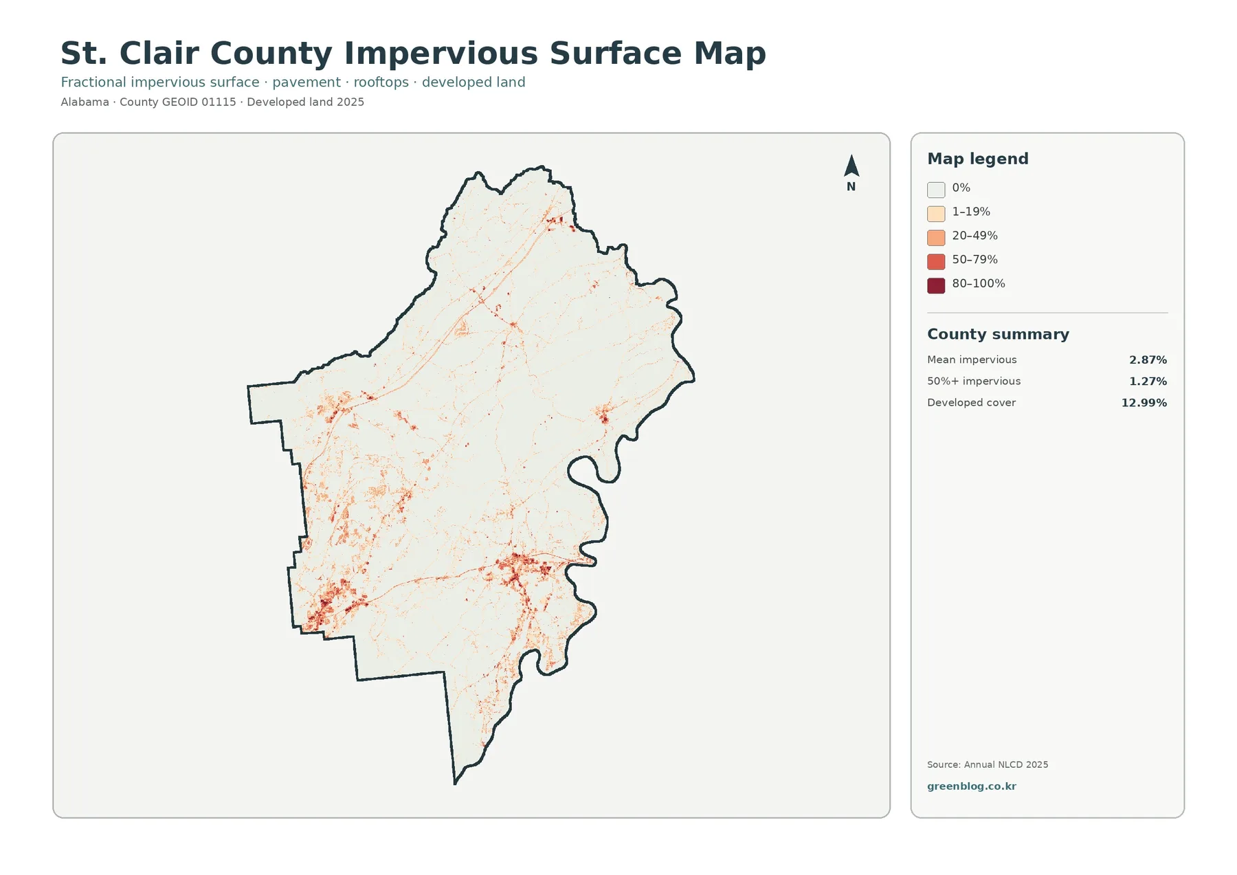
Impervious surface means ground covered by materials such as pavement and rooftops that do not absorb water as easily as soil or vegetation. The countywide mean is 2.87%, while only 1.27% of the mapped area falls in cells that are at least 50% impervious. Those values are much lower than the 12.99% developed-cover figure because a developed land-cover class can still contain yards, scattered trees, open grass, and other permeable surfaces.

The strongest impervious concentrations appear in two broad southern zones. One lies near the southwestern side of the county, closer to the Birmingham metropolitan edge, and another is centered around the Pell City area near Logan Martin Lake. Smaller red and orange clusters extend outward along transportation and settlement corridors. Farther into the forested interior, most cells remain in the 0% or 1–19% ranges, so the contrast between built places and the wooded county background is much sharper here than on the general land-cover map.

This view is especially helpful when discussing stormwater or watershed context because developed land and impervious cover are not interchangeable. A suburban neighborhood may be classified as developed across a fairly large area, yet its actual paved fraction can remain modest. The map can identify where hard surfaces are concentrated, but it cannot calculate local runoff, drainage capacity, flood depth, or erosion risk by itself. Rainfall, slope, soil, drainage systems, and current engineering information would also be needed.

What the 2025 land-cover classes say about the county as a whole

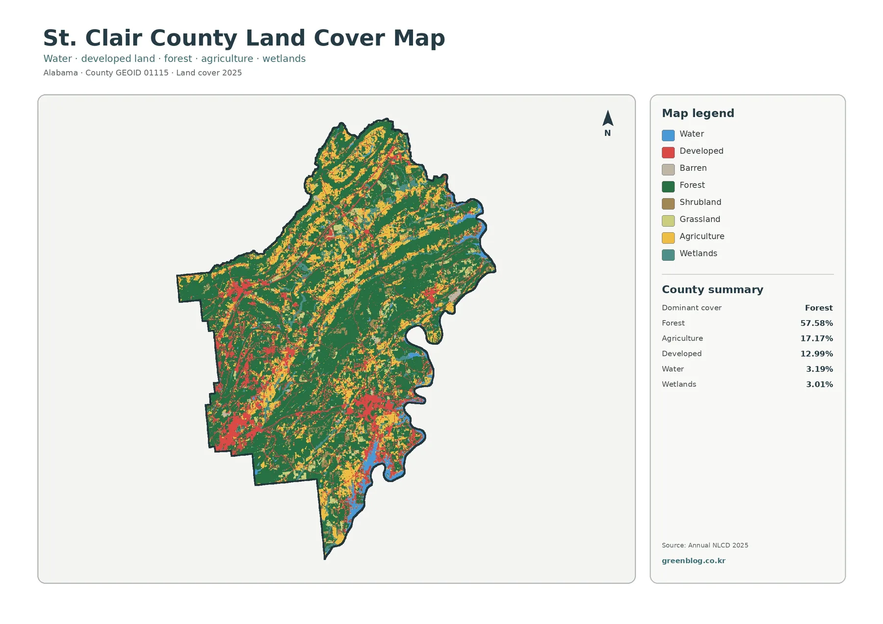
Forest is the dominant class at 57.58%, and the map makes that majority easy to see. Dark green covers large continuous areas through the center and east, while the northern half contains more frequent yellow agricultural bands. The forest is not an unbroken block; developed areas, farm fields, open vegetation, water, and wetlands interrupt it in many places. Still, the county’s overall visual character remains much greener than the developed clusters suggest when viewed alone.

Agriculture accounts for 17.17% of the 2025 classification. It is particularly noticeable across the north, where yellow patches and strips recur between forested areas, but smaller agricultural areas also appear through the central and southern parts of the county. This is a land-cover category, not a legal statement about agricultural zoning or ownership. A mapped agricultural cell describes what the surface was classified as during the observation period; it does not establish how a parcel may legally be used.

Developed land covers 12.99%. The general map broadens the urban picture beyond the highly impervious spots by showing lower-density developed classes as well. Red areas are prominent in the southwest and around Pell City, while narrower developed traces connect other settlements. Comparing this map with the impervious view is important: the developed class tells you where the landscape has a built character, whereas imperviousness estimates how much of each cell is actually covered by hard surfaces.

Water represents 3.19% and wetlands 3.01%. Those percentages are modest countywide, but the blue and blue-green classes form long, recognizable shapes along the east and southeast. Logan Martin Lake is especially conspicuous near Pell City, and the Coosa River system defines much of the eastern setting. A land-cover map can show where those water-related classes occur, but it is not a navigation chart, bathymetric map, regulatory wetland delineation, or flood-hazard map.

The forest-and-farmland map reveals the northern mosaic

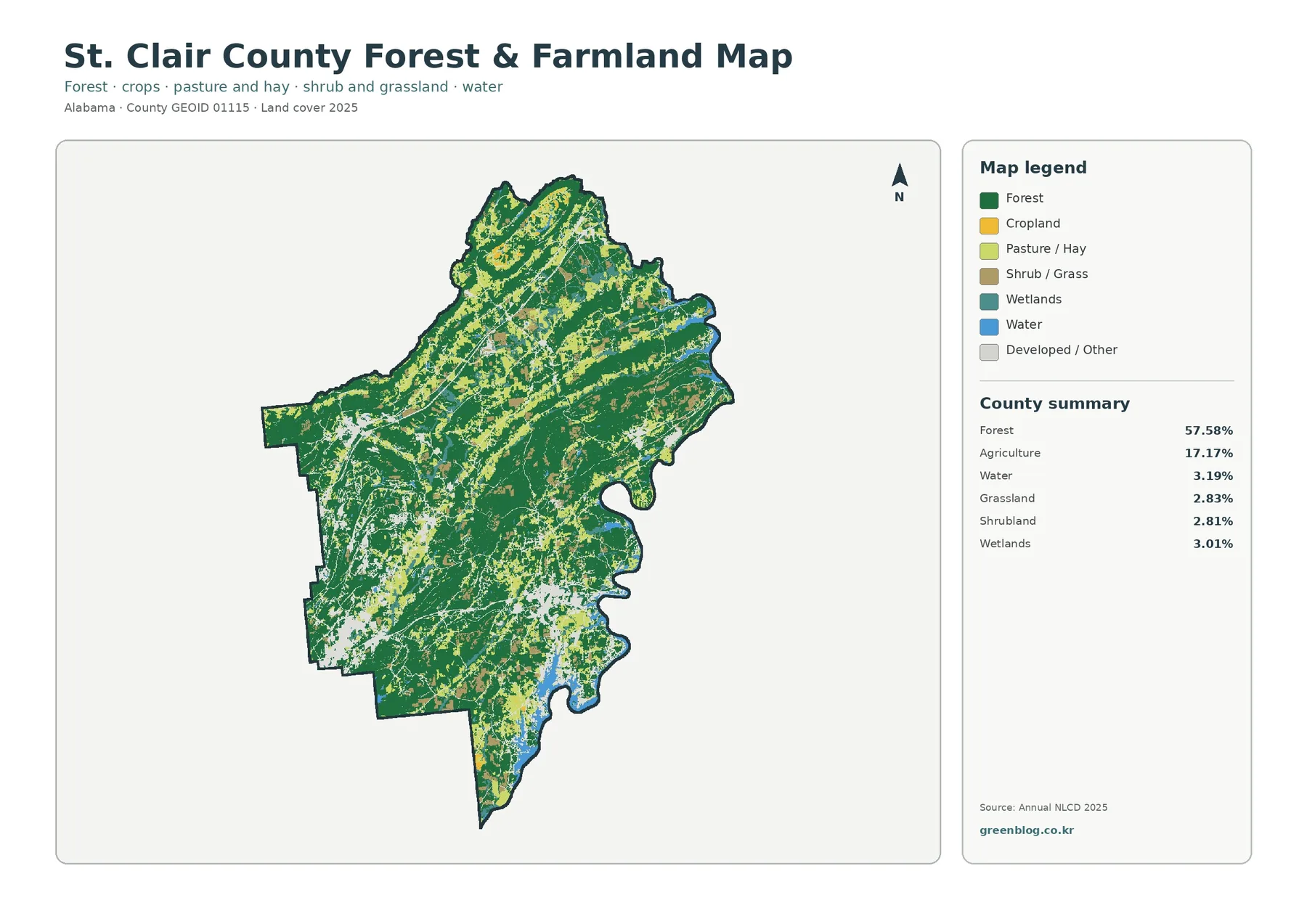
The forest-and-farmland view changes the emphasis. With most developed areas pushed into a pale background, the north becomes a patchwork of dark-green forest, lighter pasture or hay, and smaller crop areas. The central and eastern sections retain larger forest blocks. That contrast is useful for explaining why the county’s 57.58% forest share can coexist with a substantial 17.17% agricultural share: the two classes are interwoven rather than separated into a simple north-versus-south split.

Grassland is listed at 2.83% and shrubland at 2.81%. Neither class dominates the county, but both help describe the transition between woods, fields, and developed places. Small areas of low vegetation can represent several real-world conditions, so the class should not automatically be interpreted as a specific farm type, pasture condition, or planned open space. The best reading comes from comparing those cells with the surrounding forest, agricultural classes, and visible water features.

The eastern lake and river margin also stands out in this simplified view. Wetlands occur close to forest and open water in several sections, giving students and map users a clearer picture of how riparian and reservoir-edge cover differs from the upland interior. Narrow stream corridors and small wet patches may be generalized or missed at the dataset’s raster scale, so detailed habitat or wetland work should use finer local mapping and field information rather than this countywide image alone.

Reading 1985–2025 change without confusing it with a development rate

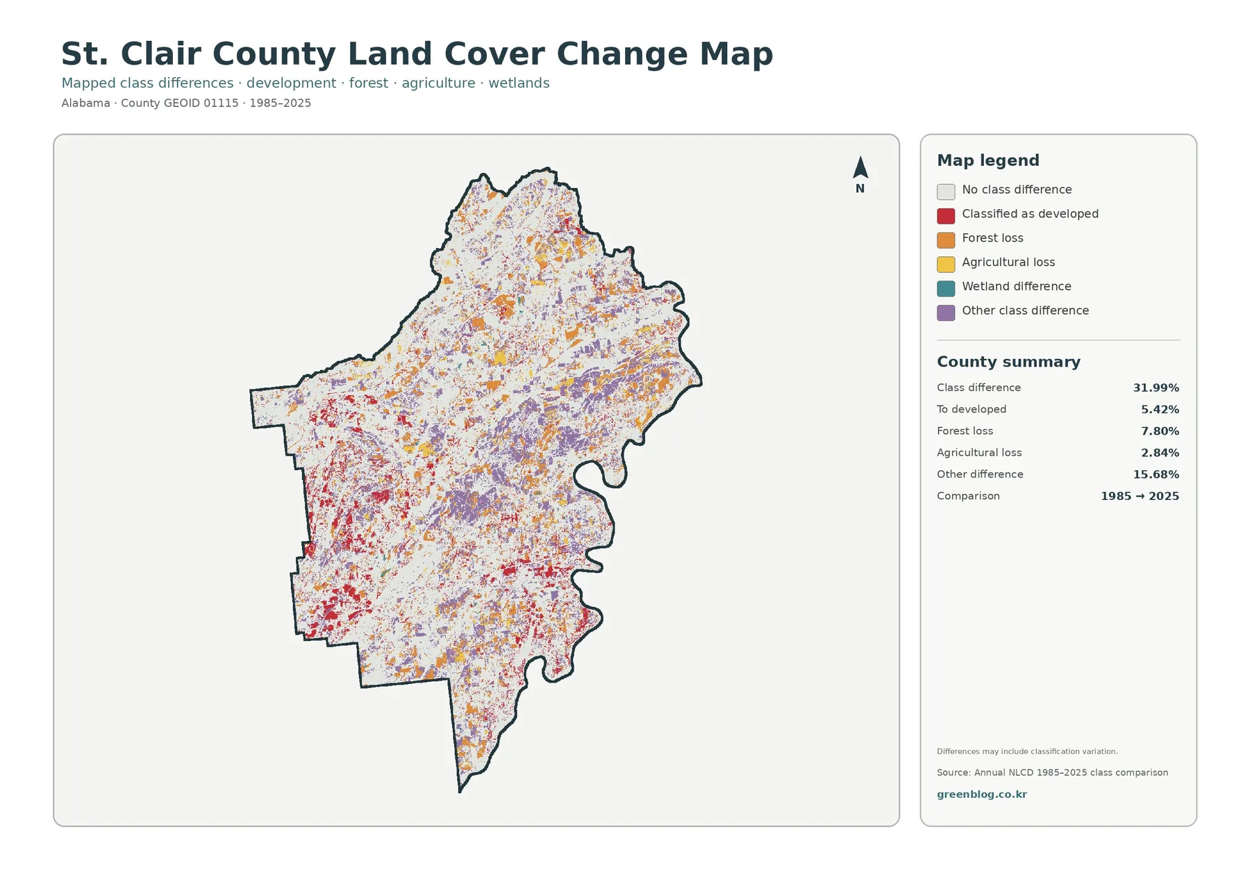
The headline value on this map is a 31.99% class difference between 1985 and 2025. It should not be read as “31.99% developed.” The map reports 5.42% as change to developed, 7.80% as forest loss, 2.84% as agricultural loss, and 15.68% as other class difference, with wetland differences shown separately in the legend. The total difference therefore combines several kinds of mapped change rather than describing one single process.

Red change-to-developed cells are especially noticeable in the southwest and through parts of the south and southeast. Orange forest-loss cells and purple other differences are spread more widely, including broad sections of the north and center. The northern landscape is particularly mixed, with many small patches of different colors. That pattern indicates a complex set of class transitions over four decades rather than a uniform conversion from forest or agriculture into urban land.

The map itself warns that differences may include classification variation. Satellite observations from different years can be affected by seasonal conditions, sensor changes, class definitions, and the way a 30-meter cell contains more than one surface type. A change-colored cell is therefore a useful place to investigate further, not final proof of a specific clearing, construction date, wetland loss, or land-management action. Historical aerial photography and local records are better tools for confirming site-level events.

Pell City, Logan Martin Lake, and the eastern water edge

The county’s official Pell City page places the city on Interstate 20 and U.S. Highway 231 beside Logan Martin Lake. That geography explains why the southeast is a useful place to compare all four maps. On the general land-cover image, developed red areas sit beside blue water and broad green forest. The impervious map then narrows attention to the harder built surfaces inside that developed zone. The change map adds a time comparison, showing which cells were classified differently between 1985 and 2025.

The same method works along the broader Coosa River edge. Start with open water to establish the shoreline, then look for wetlands near the margin, forest just inland, and developed clusters around communities. This sequence is more informative than assuming every lakeside area has the same character. Some sections remain heavily wooded, while others contain a closer mix of housing, roads, open water, and wetland classes. Countywide percentages alone cannot show those local contrasts.

Choosing the right view for a class, presentation, or county comparison

• For an overall county profile: use the full land-cover map to compare forest, agriculture, development, water, and wetlands.
• For rural landscape questions: use the forest-and-farmland map to separate wooded blocks from cropland, pasture or hay, shrub, and grass.
• For built-surface questions: use the impervious map to see where pavement and rooftops are concentrated rather than relying only on the broad developed class.
• For a historical comparison: use the class-difference map to locate changed cells, then verify important sites with additional imagery or records.

A classroom exercise can start by asking students to predict where the highest impervious values should occur after looking only at the general map. The second map can then reveal whether agricultural areas are mostly cropland or a wider mix of pasture and open vegetation. Finally, the change map can be used to test whether today’s developed clusters correspond to places with mapped change-to-developed cells. This approach encourages comparison among maps instead of treating one image as a complete explanation.

For presentations, the map pair should match the question. A watershed slide benefits from the full land-cover and impervious views, because water, wetlands, vegetation, and hard surfaces can be discussed together. A rural-landscape slide works better with the forest-and-farmland image plus the change map. When comparing St. Clair County with another county, use the percentages as a starting point, but also compare where each class is concentrated; two counties with similar forest shares can have very different settlement and water patterns.

What the 30-meter raster can and cannot tell you

Annual NLCD is designed for consistent regional and national comparison. Its land-cover information is represented as raster cells, which are small square grid units rather than legal parcels. At roughly 30 meters, one cell may contain a road, tree cover, lawn, and part of a building at the same time. The classification assigns a representative value, so narrow roads, tiny ponds, forest edges, and thin wetland strips can be simplified. This is often called a mixed-pixel effect.

Land cover also differs from zoning and land use. The St. Clair County Alabama Land Cover Map tells you what kind of surface the satellite-based classification detected, not who owns it, whether construction is allowed, or how a parcel is taxed. It is a strong tool for broad questions such as “Where is forest most continuous?” or “Which part of the county has more built surface?” It is not a substitute for a survey, wetland delineation, engineering plan, planning map, or title record.

Download the four St. Clair County land-cover JPG maps

The downloadable JPGs preserve the package’s original dimensions and are better suited than the web previews for placing into documents or slides. The manifest does not mark these 2480 × 1754 files as meeting an A3 high-resolution reference, so large-format printing should be tested before producing a final poster. Print quality depends on the physical size, printer, scaling, and viewing distance, while map classification quality depends on the source data and raster method.

Frequently Asked Questions

Related Maps

• Autauga County Alabama Land Cover Map
• Baldwin County Alabama Land Cover Map
• Barbour County Alabama Land Cover Map

Sources

• MRLC Annual NLCD Data — land-cover, developed-cover, and impervious-surface datasets
• USGS Annual NLCD Land Cover Classification — class definitions and interpretation
• U.S. Census Bureau TIGER/Line Shapefiles — county boundary reference
• St. Clair County official Travel Guide — county geography, the Coosa River, Logan Martin and Neely Henry dams, I-20, and I-59
• St. Clair County official Pell City page — Pell City, Logan Martin Lake, I-20, and U.S. 231 context