Okeechobee County Florida Land Cover Map: Farms Around a Wetland-Lake Landscape

The Okeechobee County Florida Land Cover Map is dominated by agricultural land, but the county is not simply one large farm belt. The supplied 2025 summary reports agriculture at 46.84%, wetlands at 28.66%, water at 12.12%, developed land at 5.11%, shrubland at 4.38%, forest at 2.64%, and grassland at 0.16%. On the map, broad agricultural areas occupy much of the interior while wetlands interrupt them repeatedly, and the large water area along the south creates a very different edge.

This page compares four related views: 2025 land cover, forest and farmland, impervious surface and developed land, and a 1985–2025 land-cover difference map. The WebP images are intended for quick on-page comparison, while the four original JPG maps are available together in one ZIP download. Using the views side by side makes it easier to separate current surface cover from hard-surface intensity and from long-term classification differences.

Agriculture covers nearly half of the county, but wetlands break up the interior

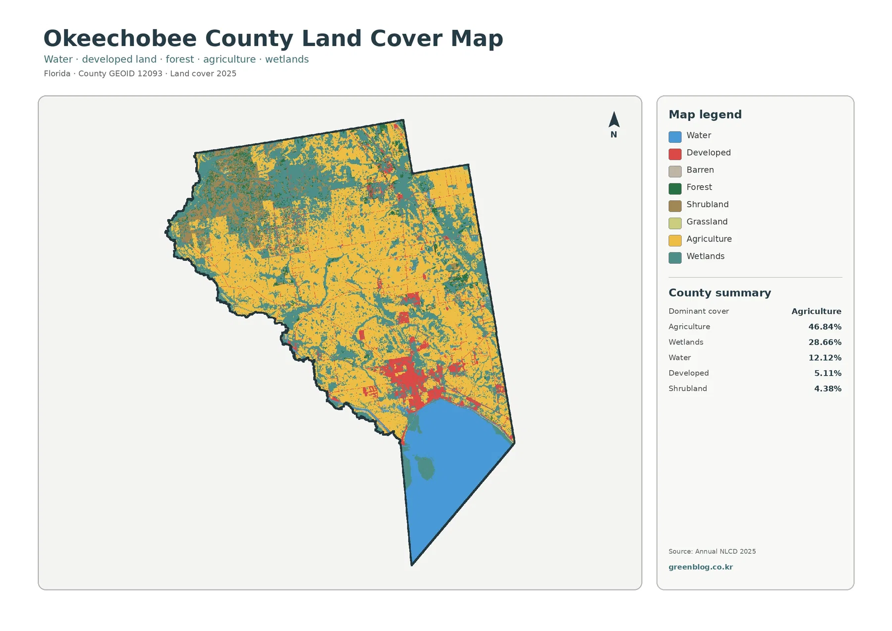
Agricultural color extends across much of the center, east, and north of the county. It is not a perfectly continuous field of one use; wet areas, small forested areas, developed surfaces, and other classes interrupt it. Even so, the 46.84% summary value is large enough to define the countywide view. Agriculture is the first category to understand before moving to the more localized developed areas or the smaller forest share.

Wetlands are the second-largest class at 28.66%. They appear broadly in the west and northwest and continue through other parts of the county in bands and irregular areas between agricultural cover. The important point is not simply that agriculture ranks first and wetlands second. Their close proximity across much of the map creates a mixed agricultural-and-wet landscape rather than two cleanly separated zones.

Water accounts for 12.12% of the supplied summary, and the most obvious water area is along the southern part of the county where the boundary reaches Lake Okeechobee. The South Florida Water Management District describes the lake as a central freshwater resource within the larger Kissimmee-Okeechobee-Everglades system. This land-cover map does not show lake operations, depth, or water quality, but the large blue area provides essential context for the county’s surface pattern.

Developed land is only 5.11%, yet a concentrated red area in the south-central part of the county stands out because surrounding agriculture and wetlands use much softer colors. Okeechobee County’s official site identifies the City of Okeechobee as the county’s only incorporated area. The land-cover map can be used to see the broader developed concentration around that part of the county, although land-cover pixels cannot be substituted for municipal or zoning boundaries.

Land cover describes the ground surface, not ownership or legal land use

It is especially important to keep the meaning of land cover clear in Okeechobee County because agricultural and wetland colors sit next to each other over large areas. Land cover classifies what is covering the ground as interpreted from remotely sensed data. It does not identify the owner, the legal use of a parcel, the zoning designation, or whether development is permitted.

An agricultural cell may represent different kinds of working land and may include smaller features that are not separately mapped at county scale. A wetland cell is not automatically a regulatory wetland boundary, and a developed cell can contain grass, trees, bare ground, and pavement in the same general area. Those distinctions matter when the map is used in a report or classroom presentation, because the colors should not be presented as parcel-level facts.

The forest-and-farmland view makes Okeechobee’s working landscape easier to compare

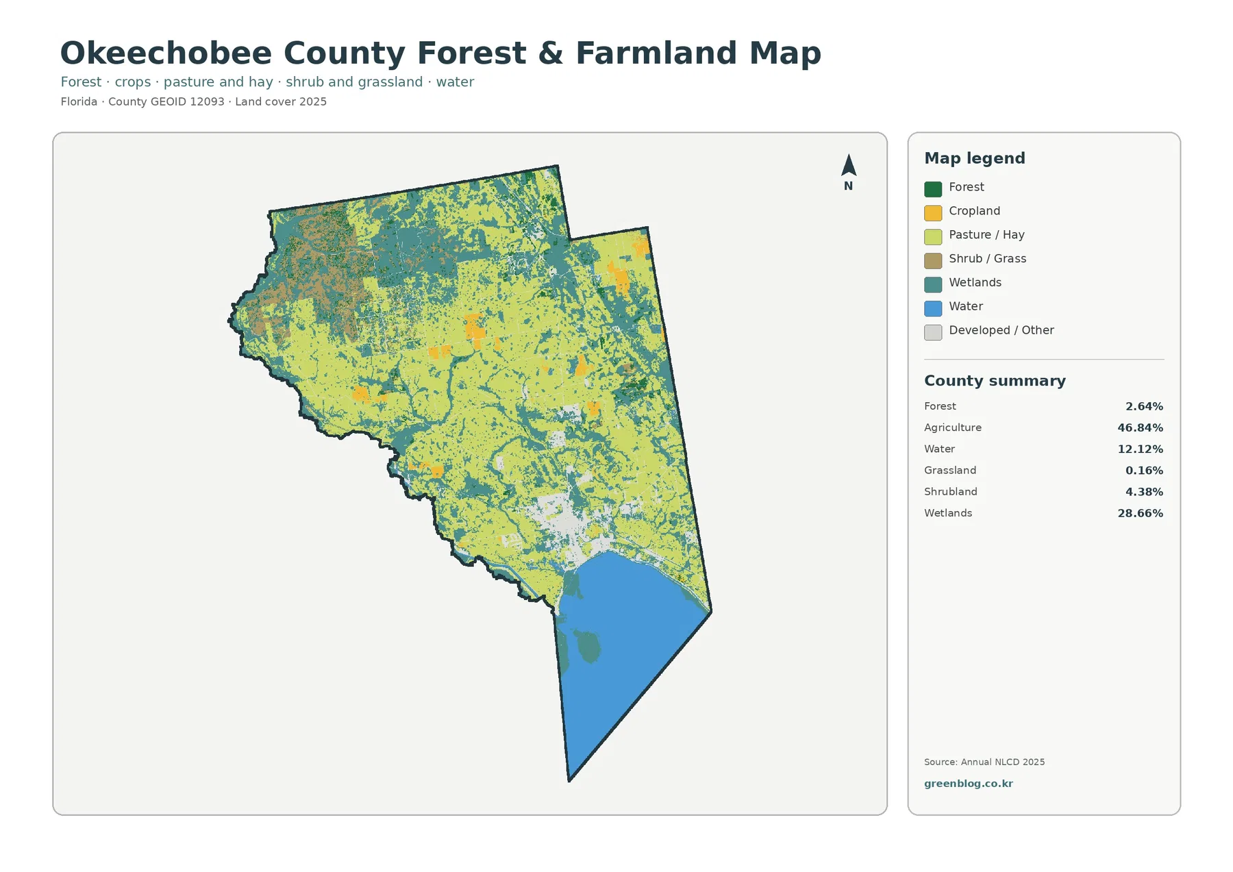
Removing some of the competing land-cover colors makes the dominance of agriculture even easier to see. Agricultural classes spread through the central and eastern county and continue northward, while wetlands repeatedly occupy the spaces between them. This focused view is useful when a reader wants to discuss working land without letting the more visually intense developed category dominate the page.

Forest is only 2.64% in the supplied county summary. Dark green areas are visible in the north and northwest and in smaller locations elsewhere, but they do not form one broad countywide forest block. That is a meaningful local contrast: Okeechobee County’s map is shaped far more by agriculture and wetlands than by forest. Comparing it with forest-dominant Florida counties should therefore use both the percentage and the actual arrangement on the map.

Shrubland is 4.38% and grassland is listed at 0.16%. The very small grassland value should not be interpreted as meaning that almost no grassy surfaces exist on the ground. Agricultural classification can include pasture and hay areas, and a raster cell receives one dominant class even when several surface types occur within it. The map summarizes broad cover, not every fence line, pasture edge, drainage feature, or tree row.

For agricultural presentations, the focused map works best as a county-scale reference. It can show where working land is extensive and how it meets wetlands and water, but it does not identify farm ownership, crop type, stocking rates, or current production. Those questions need agricultural records or site-specific information. The map’s strength is showing the relationship among broad surface classes in one consistent frame.

Lake Okeechobee water and inland wetlands need to be read as separate classes

The difference between 12.12% water and 28.66% wetlands is central to understanding this county. Open water is shown separately from wetland surfaces that may support vegetation and may be seasonally or persistently wet. The large southern blue area is visually obvious, while the inland wetlands appear in a different color and spread through agricultural parts of the county. Treating all of those areas as simply “water” would erase a major part of the map’s information.

The South Florida Water Management District places Lake Okeechobee and its surrounding watershed within the larger Greater Everglades system. That official context helps explain why a county map that combines agriculture, wetlands, and lake water is useful for watershed education. It does not, however, turn the land-cover map into a hydrology or regulatory product. Flood levels, drainage direction, wetland jurisdiction, water quality, and canal operations require different data.

Hard surfaces are concentrated even though developed land is easy to notice

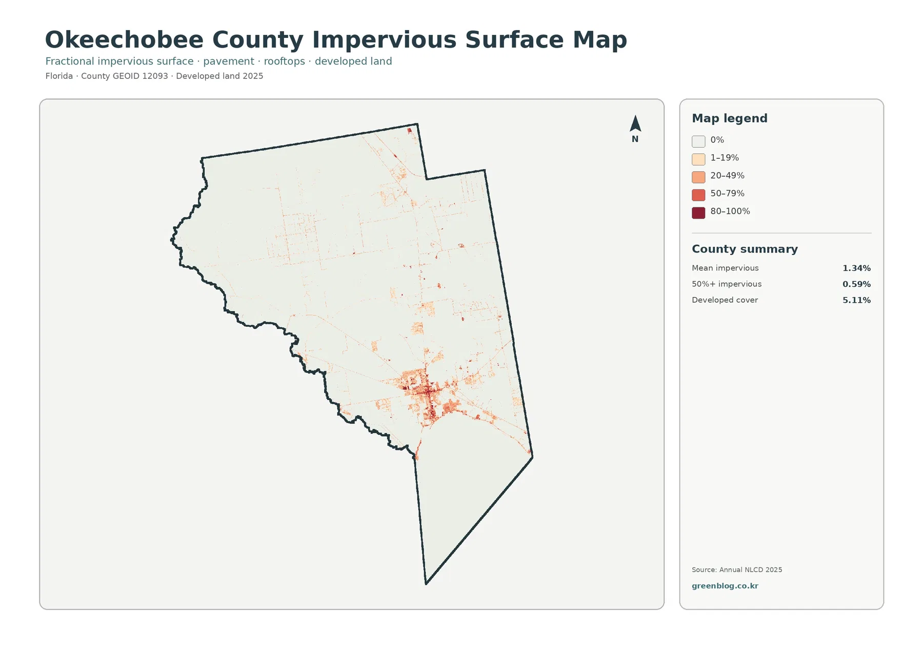
The impervious map tells a more concentrated development story than the general land-cover map. Most of the county remains near the lightest end of the scale. The strongest values cluster in the south-central developed area, while thin traces and smaller concentrations extend through other parts of the county. Mean impervious cover is just 1.34%, and 0.59% of the county is mapped at 50% or greater impervious surface.

Those values are much lower than the 5.11% developed-land share because the measures are not interchangeable. Developed land is a broader land-cover category that can include lawns, tree cover, open space, and other permeable surfaces around buildings and roads. Impervious cover isolates the proportion occupied by hard materials such as pavement and rooftops. A developed area therefore does not need to be mostly paved.

The narrow lines visible on the impervious map may resemble roads, but this should not be treated as a transportation map. It does not supply road names, lane counts, traffic levels, or pavement conditions. If a project needs transportation detail, a road layer should be consulted separately. The impervious image is most useful for showing where hard surface is concentrated relative to the county’s much larger agricultural and wetland areas.

The 1985–2025 comparison reports class differences, not a single rate of land transformation

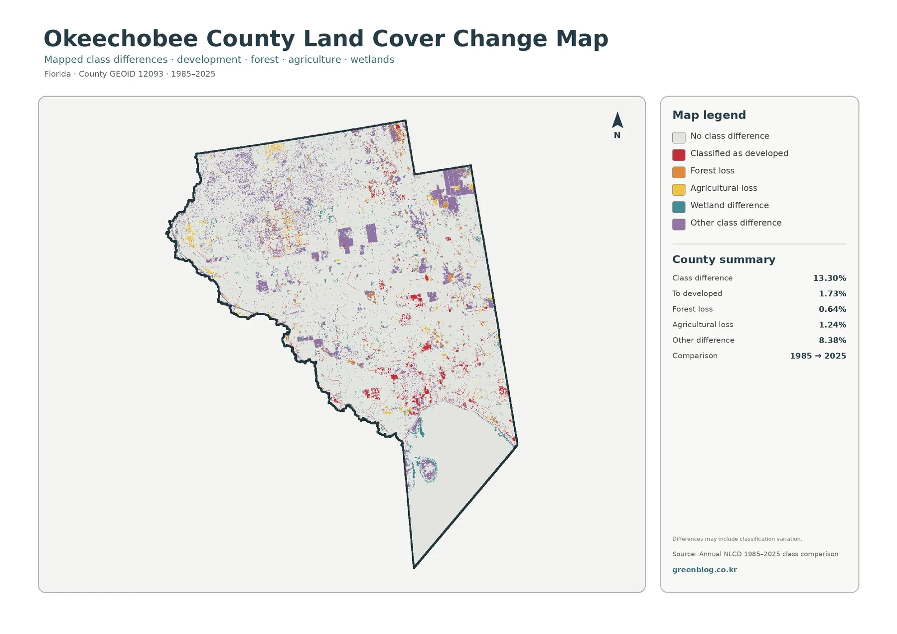
The total class difference is 13.30%. That figure should not be rewritten as “13.30% of Okeechobee County was developed” or “13.30% was permanently altered.” It is the share of cells with different classifications in the two comparison years. The map itself warns that classification variation may be included, so the number is best used to identify areas for closer review rather than to assign a cause.

The supplied summary breaks out 1.73% classified to developed, 0.64% forest loss, 1.24% agricultural loss, and 8.38% other difference. The largest named value is therefore the broad “other difference” category, not development. This is important because the map contains purple and other difference colors across the north, east, and interior in addition to the more familiar red development marks.

Forest-loss and agricultural-loss labels also need careful language. A cell that differs between two classifications does not reveal the cause by itself. A change might reflect actual clearing or conversion, but other factors such as imagery, seasonal conditions, mixed pixels, or differences in class assignment can matter. Intermediate-year imagery, land records, agricultural information, or local planning documents are needed before a specific explanation is stated.

A practical way to use the comparison is to place it beside the 2025 map. Red areas in the south-central county can be checked against the present developed concentration, while other difference areas farther north can be compared with current agriculture or wetlands. This turns the change map into a screening tool: it helps select places for more detailed study without pretending that the map alone proves what happened there.

Four cross-map comparisons explain the county better than one legend

The first useful comparison is agriculture versus wetlands and water. Agriculture is the largest single class at 46.84%, but wetlands and open water together exceed 40% of the supplied summary. On the map, these surfaces are interwoven rather than isolated from each other. That relationship is a more informative description of Okeechobee County than simply calling it an agricultural county.

The second comparison is developed land versus hard surface. The 5.11% developed share is visible because it is concentrated, yet the countywide mean impervious value is only 1.34%. The visual contrast explains why a small developed center can be prominent without representing a highly paved county overall. It also shows why development intensity should not be inferred from the red land-cover color alone.

The third comparison is forest versus agriculture. Forest is 2.64%, while agriculture is more than seventeen times larger by the supplied percentages. The focused vegetation map confirms that difference visually. Small wooded areas are still important for local context, but they do not control the countywide view in the way that agricultural and wet surfaces do.

The fourth comparison is current condition versus two-date difference. The 2025 maps answer what the latest supplied classification looks like. The change map answers where 1985 and 2025 classifications differ. A location can be agricultural today and still have a change history, while a location with a change symbol should not be described using that symbol as if it were a current land-cover class.

Choosing the right map for printing, teaching, and county profiles

For a general county profile, start with the 2025 overview because it places the 46.84% agricultural share, the 28.66% wetland share, Lake Okeechobee water, and the concentrated developed area in one frame. It works well when the audience first needs to understand the broad balance between working land and wet environments before looking at a specialized theme.

For agriculture or natural-resource education, the forest-and-farmland view reduces visual competition and makes the agricultural-wetland relationship easier to discuss. For development topics, the impervious map is more useful because it separates hard surface from the broader developed category. For historical comparison, the change map should be paired with a current map so that the audience can distinguish present cover from two-date differences.

The original JPG files measure 2480×1754 pixels. They are suitable for ordinary print layouts, slides, and digital reference, but the package does not mark them as meeting the A3 high-resolution reference. Enlarging the files can make the existing pixels larger, not add missing source detail. Tiny drainage features, narrow roads, buildings, and parcel boundaries therefore require more detailed source data when they matter to the project.

Raster cells, observation dates, and local planning data set the map’s limits

Annual NLCD is a raster classification, which means the landscape is represented by cells assigned to dominant classes. A real cell can contain vegetation, pavement, soil, standing water, and other surfaces at the same time. Edges between agriculture and wetlands or between developed land and fields are especially likely to be more complex on the ground than the clean color boundary suggests.

The 2025 map is tied to its supplied observation and classification year. Construction, agricultural changes, vegetation recovery, or changes in water conditions after that point may not appear. The 1985–2025 map is also a two-date comparison rather than a year-by-year record. A place could change several times between those dates and end in a class similar to its starting condition.

These limits define the right use rather than making the maps unhelpful. They are strong tools for county-scale comparison, selecting areas for further research, classroom explanation, and presentation graphics. Okeechobee County provides separate zoning and future land-use resources for legal planning questions. Those products should remain separate from land-cover classification when a decision concerns a specific property or permitted use.

Frequently Asked Questions

Sources and Reference Data

• MRLC Annual NLCD Data – source information for the 2025 land-cover and 1985–2025 comparison products.
• USGS Annual NLCD Land Cover Classification – official descriptions of developed, forest, agricultural, wetland, and other classes.
• U.S. Census Bureau TIGER/Line Shapefiles – official geographic boundary reference for Okeechobee County.
• Okeechobee County – About the County – official county context, including information about the City of Okeechobee.
• South Florida Water Management District – Lake Okeechobee – official context for Lake Okeechobee and its watershed.

Related Maps

• Alachua County Florida Land Cover Map
• Baker County Florida Land Cover Map
• Bay County Florida Land Cover Map