Across much of Boone County, Indiana, rectangular farm fields occupy the landscape. Two places stand apart on the 2025 land-cover map: a compact developed center around Lebanon and a larger patchwork of developed land toward Zionsville and Whitestown in the southeast. Agriculture accounts for 77.57% of the countywide classification, yet that single number does not capture the contrast between its rural interior and the southern edge of the Indianapolis metropolitan area.
The Boone County Indiana Land Cover Map collection brings together four views of this landscape: current cover, forest and farmland, impervious surfaces, and differences between 1985 and 2025. You can explore the WebP previews here and download the four original JPG maps in one ZIP. Each explanation distinguishes what the colors show from what they cannot establish, then suggests a suitable image for reports or presentations.
Table of Contents
Why Lebanon and the southeast stand out against farmland
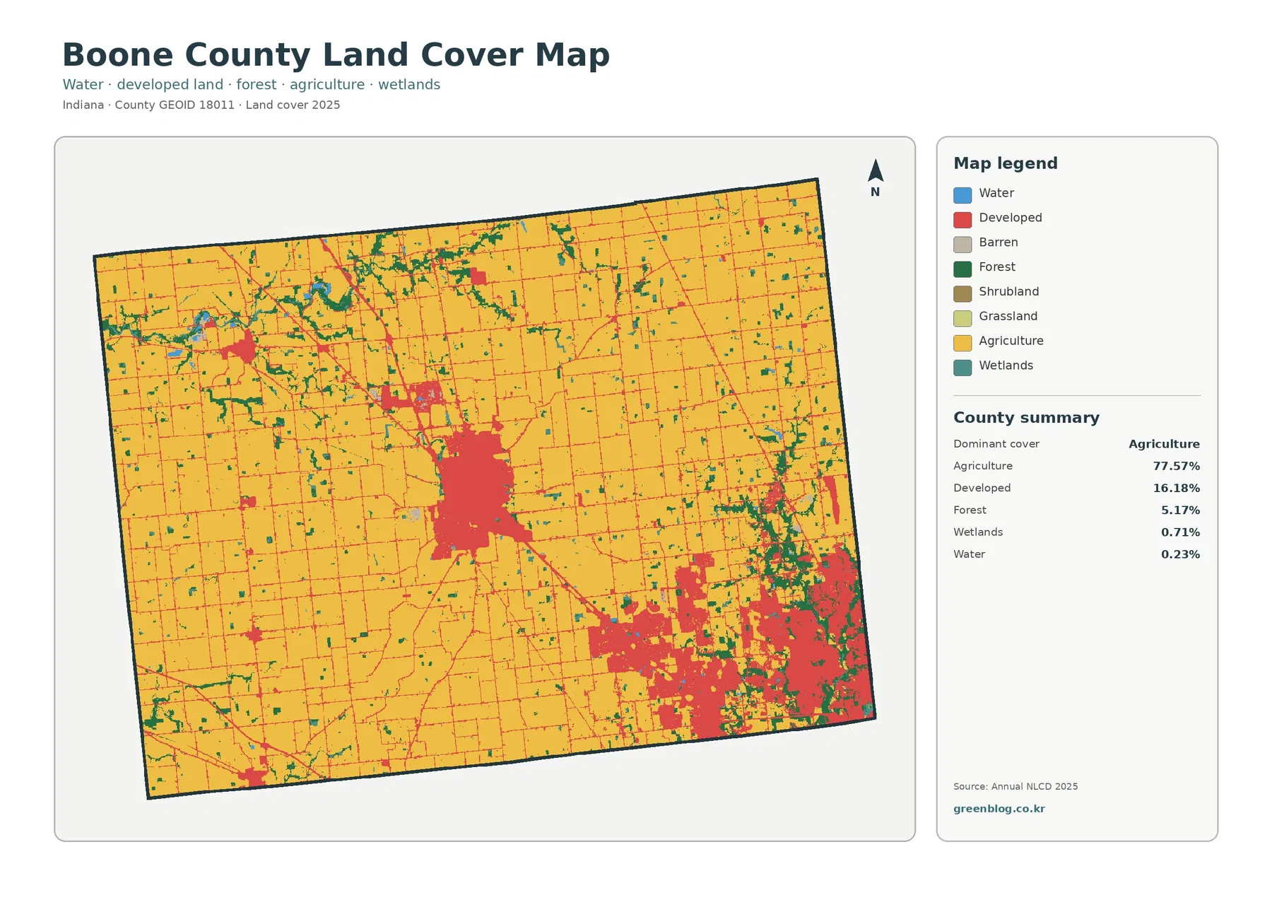
Start with the broad yellow areas on the general map. They cover most of the northern and western parts of Boone County, continue around smaller settlements, and reach close to Lebanon’s developed center. Yellow represents agricultural land cover, not a legal agricultural district. County figures assign 77.57% to agriculture, 16.18% to developed cover, and 5.17% to forest. Water and wetlands occupy much smaller shares, 0.23% and 0.71% respectively.
Lebanon is easy to find near the center because the red developed cells form a recognizable concentration amid surrounding fields. Further southeast, red covers a wider and more irregular area. Pockets of vegetation and other surface classes interrupt that red cover, preventing a solid block. That difference in shape matters: a large contiguous urban footprint can contain parks, lawns, stream corridors, and undeveloped parcels, even when development is its most noticeable feature.
Smaller red marks in the northwest provide another useful comparison. Their general position is consistent with the area around Thorntown, although the picture has no municipal boundaries or printed road labels. Farm lanes, commercial sites, and settlement edges can also appear as small developed features. Use a separate county road or boundary layer before identifying any individual dot with a particular town or property.
County transportation documents describe Lebanon, Whitestown, and Zionsville as distinct places within a network of roads and growing communities. It also places the county northwest of Indianapolis. Those details help readers orient the large southeastern developed area, but they are not evidence that every red cell belongs to one municipality. Surface cover, municipal boundaries, and legal zoning come from different datasets and should not be treated as interchangeable.
If you are creating a simple county overview, keep this first map visible while reading the others. Its main strength is context: viewers can see where agriculture still dominates and where built surfaces interrupt it. Comparisons with the remaining three images add detail without replacing that countywide context.
Roofs, pavement, and the developed clusters they reveal
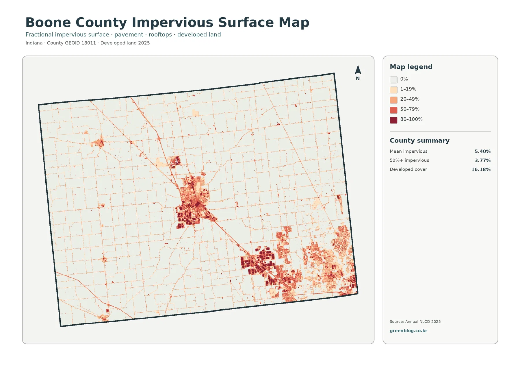
Dark spots on the impervious-surface map mark places where water has difficulty soaking into the ground, such as roofs, paved streets, and parking areas. Boone County has a mean mapped impervious value of 5.40%, while the area in the 50%-or-higher impervious category is 3.77%. Neither measure is interchangeable with the 16.18% developed-land share on the first map.
Even neighborhoods full of streets and buildings contain lawns, trees, bare soil, and other open spaces. A developed classification does not mean the entire neighborhood is paved. Viewed together, these maps describe two sides of the same place: its overall cover class and the intensity of hard surfaces. Seeing them together prevents an overly simple assumption that every developed cell is covered in concrete.
Around Lebanon, the darker impervious patches sit within a compact central concentration. Several dense clusters appear again in the county’s southeast, where a larger urbanized area borders agricultural land. Farther north and west, lighter colors dominate, interrupted mainly by thin traces and isolated dark marks. These are useful patterns for comparing a rural road network with more concentrated built surfaces, but the traces do not supply names or traffic volumes.
Mean imperviousness summarizes the entire county, including vast areas with little pavement. That is why it can remain at 5.40% even when the southeastern image contains strongly colored developed pockets. During a classroom comparison, put this image beside the general cover view and identify developed areas with high impervious intensity. Impervious intensity varies even within a single developed cluster.
When considering drainage, treat the pavement pattern as a starting clue rather than a flood forecast. Runoff also depends on rainfall, slopes, soil characteristics, ditches, pipes, streams, and local maintenance. No single pavement image accounts for every aspect of local drainage. Owners evaluating a particular property should consult current drainage, elevation, and floodplain records instead of relying on one dark cell.
Field blocks, narrow woods, and waterways around them
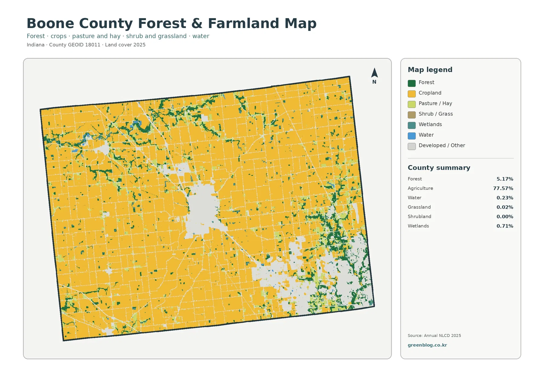
Removing the emphasis on roads and buildings brings Boone County’s agricultural pattern into sharper focus. Broad crop-colored blocks dominate the forest-and-farmland view across the north, west, and rural central area. Woodland is not concentrated into one enormous forest. Instead, green patches and narrow strips appear among the fields, occasionally forming more irregular shapes near channels and settlement edges.
Field continuity changes noticeably as the view approaches the county’s settled areas. Lebanon appears as a conspicuous break in the surrounding crop-colored area. Southeastern development divides farmland into smaller pieces, with green patches mixed among built areas. This contrast is worth showing in an agricultural presentation: the countywide crop share may be high, but the shape and continuity of the field area are not uniform everywhere.
Countywide figures identify 5.17% forest, 0.71% wetlands, 0.02% grassland, and 0.23% water. Shrubland is displayed as 0.00% at the summary’s level of rounding. These smaller categories should not be inflated into large habitats that the map does not depict. Even these small categories help locate breaks in the cultivated landscape and areas worth checking on more detailed environmental maps.
Purdue Extension’s Boone County agriculture materials provide a separate local perspective. Purdue’s account cites 85% of county land in farms in the 2017 Census of Agriculture and describes the local importance of corn and soybeans. That 2017 farm statistic is not a competing estimate of 2025 agricultural cover. Inclusion in a farm and classification as agricultural ground cover measure different things in different years. Side-by-side comparisons work only when those definitions are stated clearly.
Notice how straight many of the field boundaries appear. Straight field edges make the image easy to interpret, but they are not surveyed parcel lines. Raster land-cover products assign a category to a grid cell; a field edge, tree row, ditch, or farm building may occupy only part of that cell. Property limits, crop-specific acreage, drainage easements, and ownership require more detailed records.
Small water and wetland features deserve special care when reading the vegetation image. Narrow green or blue marks can follow drainage corridors, but the preview cannot establish perennial flow or legally protected wetlands on any parcel. It gives a regional clue that can guide further research. Regulatory determinations require an agency delineation and current site-specific information.
What the 1985–2025 comparison can—and cannot—date
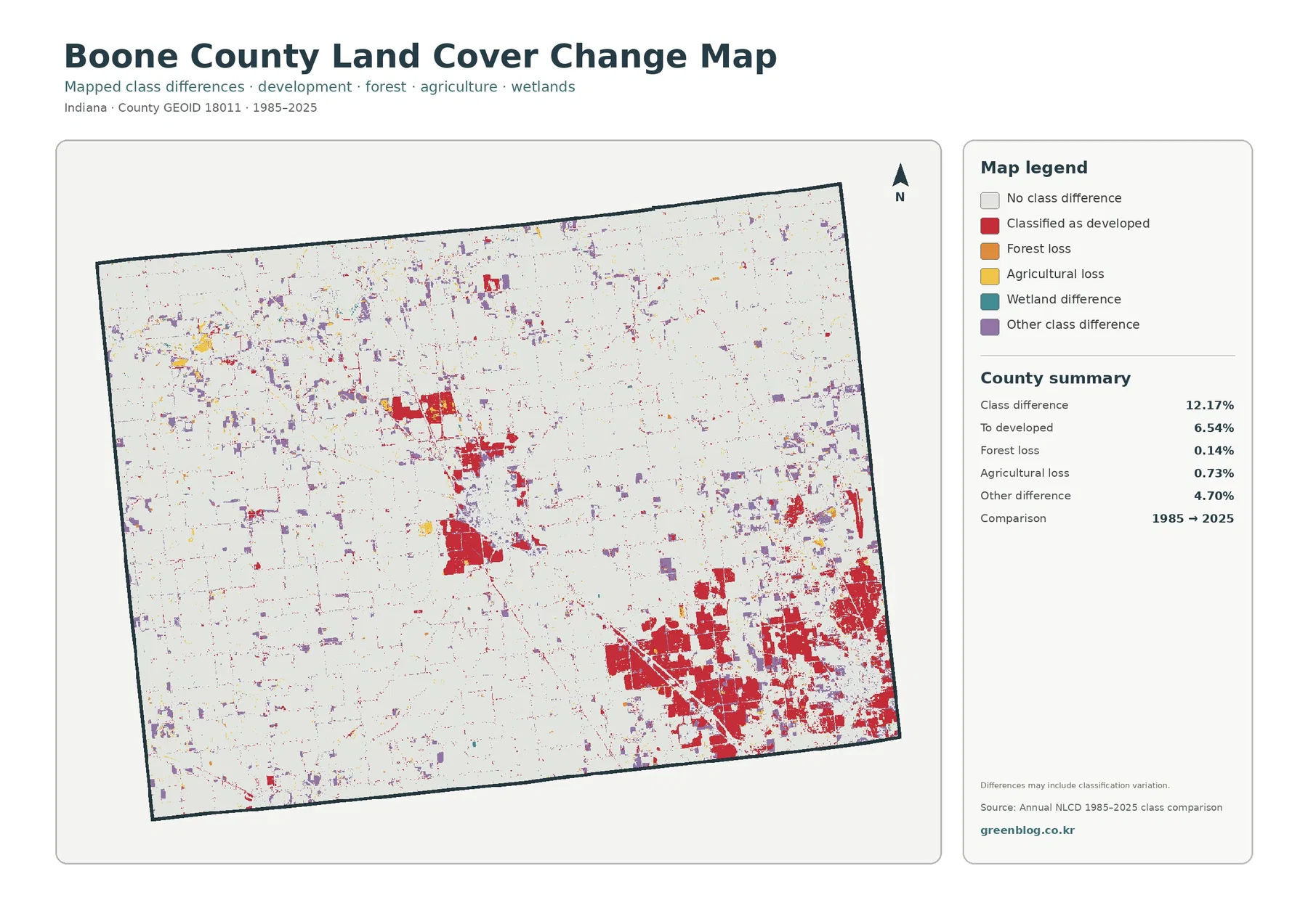
Rather than depicting new buildings alone, the final image compares changes in classified ground cover. Its two comparison dates are 1985 and 2025. Boone County’s supplied summary reports 12.17% overall class difference. Category figures break that result into 6.54% conversion to developed cover, 0.14% forest loss, 0.73% agricultural loss, and 4.70% other difference. Wetland difference has a legend entry but no separately stated percentage in this summary.
Developed-conversion red is especially noticeable in the southeast. Similar red marks occur around Lebanon and at smaller developed clusters elsewhere in the county. Other-difference purple marks are distributed more widely, including scattered spots across farmland in the northern and western parts of the county. Development-related differences form noticeable concentrations, whereas other changes are more scattered and harder to see at this map scale.
Red change cells mark places assigned different classes at the two endpoints, with developed cover at the later date. Construction dates cannot be recovered from a red change cell. Nor can it tell you whether a particular change involved homes, warehouses, roads, or another type of development. Project names, permits, and construction timelines are absent from this raster comparison. Historical aerial imagery and local records are necessary to answer those questions.
Yellow and orange classes on the change legend also require careful interpretation. Both colors flag changes involving agricultural or forest classes; neither explains why a particular field or stand of trees changed. Farming practices, construction, flooding, seasonal imagery, and classification uncertainty can each call for investigation. Avoid presenting a color as proof of a specific cause when the source is a two-date classification comparison.
Most importantly, 12.17% is not a measure of land ‘lost’ to urbanization. Several kinds of mapped difference contribute to the total. Sites that changed during those decades but returned to their original class at the end may show no endpoint difference. Readers interested in the present landscape should begin with the 2025 overview and turn to this historical map only after they understand the current pattern.
Choose a map based on your question, not its brightest colors
Someone preparing an overview of Boone County’s economy or rural setting can use the general land-cover map as a starting image. Despite agriculture’s countywide lead, Lebanon and the southeastern developed clusters keep the landscape from looking uniform. Adding a small legend explanation alongside the image is more helpful than listing every possible NLCD category in the caption.
To discuss Lebanon, begin by comparing the general cover and impervious-surface views. Developed cover outlines a broader footprint than the most intensely paved blocks, clarifying the difference between an urban area and its hard surfaces. Next, check the change image to see which locations differ between the two endpoints. Working in that order helps presenters avoid labeling every part of present-day Lebanon as new development.
Southeast of Lebanon, the forest-and-farmland view adds another layer of detail. Remaining fields and wooded patches become easier to distinguish from the surrounding developed mosaic. Combined with the impervious view, it shows that not every space inside an urbanized area has the same surface. At the southeastern edge, this comparison prevents a large red area from being mistaken for one continuous paved surface.
Near Thorntown in the northwest, use the general overview to orient a closer reading of small impervious traces. Small developed clusters have a different visual character from Lebanon or the southeast. If a project needs the exact outlines of municipal land or a named highway, add authoritative boundary and transport layers. These four images do not supply those precise boundaries or road identities.
Maps make strong classroom illustrations when the question stays appropriate to their scale. Students might compare the amount of agricultural cover with the distribution of high-impervious pockets or discuss where narrow wooded strips interrupt large field blocks. Regional presentations can contrast the rural interior with the developed southeastern edge. Neither exercise requires guessing at individual parcel histories.
A practical note about the JPG set and scale
Each of the four source JPGs measures 2480 × 1754 pixels. On-page images serve as previews; the ZIP contains original JPG versions of all four views: general cover, forest and farmland, impervious surfaces, and change. In a slide presentation, a full-county view followed by a companion image at the same orientation makes comparisons easier. Readers can then compare locations without learning a completely new layout.
Before printing, inspect the labels and legend at the intended page size. No A3 high-resolution print certification appears in the supplied asset manifest. Testing a print at the intended size helps determine whether the legend remains legible, especially when viewers will stand across a room. Enlarging the image artificially will not add finer geographic detail.
There are more important limits than printing size. Land-cover cells generalize complicated surfaces into categories; small features can be mixed within a cell or absent at this resolution. The 2025 observation year does not turn the map into a live record of construction activity. Boundary and property questions require more precise data, and environmental determinations require the appropriate regulatory source.
Local planning materials from Boone County’s Area Plan Commission address long-range growth and land-use regulation. Planning records address legal or policy questions that a satellite-based cover classification cannot answer. Agricultural color does not prove agricultural zoning, developed color does not establish permitted use, and wetland color is not an official wetland determination. Before decisions about purchases, construction, drainage work, or flood insurance, consult the county and appropriate agencies directly.
Questions readers ask about Boone County's map patterns
Why does the southeast look heavily developed in an agricultural county?
Countywide agriculture figures combine extensive rural fields with smaller areas of different cover. Large farmed areas in the north and west coexist with concentrated developed cover toward Zionsville and Whitestown. Even with its prominent red clusters, the southeast does not change agriculture’s countywide lead.
Does the Lebanon cluster have the same outline on the impervious map?
No. Developed classes may encompass yards, landscaping, and open space around buildings. Impervious mapping isolates pavement and roofs and distinguishes the intensity of those hard surfaces. Use both images if the question concerns the difference between urban land and hard surfaces.
Is the 12.17% difference an estimate of land newly built over during forty years?
Not by itself. Several types of endpoint classification difference make up that total. According to the supplied summary, 6.54% falls in the conversion-to-developed category. Other classes contribute to the remainder, and the two-date raster misses some changes between endpoints.
Frequently Asked Questions
If agriculture is 77.57%, why does southeast Boone County look so developed?
The 77.57% figure is a countywide share, so large farm areas in the north, west, and interior coexist with a concentrated southeastern urban footprint. Official county planning materials also place the southeast within the Indianapolis urbanized context. The land-cover image shows that concentration, but it does not define municipal boundaries or explain every development project.
Why is developed cover 16.18% when mean impervious cover is only 5.40%?
Developed land-cover classes can include lawns, trees, bare soil, and other permeable surfaces around buildings and roads. Impervious cover isolates hard materials such as rooftops, pavement, and parking areas, so its countywide mean is lower than the broader developed-class share.
Does the 12.17% class difference mean that much of the county became developed?
No. The 12.17% total includes 6.54% classified as developed plus forest loss, agricultural loss, other class difference, and wetland difference that has no separate summary percentage. It represents cells classified differently at the 1985 and 2025 endpoints, not a single development or damage measure.
Sources and local reference material
- MRLC Annual NLCD Data — official entry point for land-cover products and related resources.
- USGS Annual NLCD Land Cover Classification — category descriptions used to interpret the map legend.
- Boone County Area Plan Commission — county planning resources for checking legal and policy context.
- Purdue Extension Boone County Agriculture — county-specific agricultural background and census context.
- Boone County Thoroughfare Plan — local transportation and settlement context for interpreting the developed clusters.
Map File Information
Download one ZIP archive containing the four original land-cover map JPG files.
- Included Files: Four original land-cover map JPG files
- File Type: ZIP archive containing four JPG files
- Intended Use: Map comparison, learning, and print reference
Related Maps
- Adams County Indiana Land Cover Map
- Allen County Indiana Land Cover Map
- Bartholomew County Indiana Land Cover Map
Green Map creates custom-edited map images using open geographic data sources such as geoBoundaries, Natural Earth, OpenStreetMap, and government open data. These maps are edited visual materials, not raw data files, and are provided for education, documents, presentations, and graphic reference.