Glascock County has a distinctly mixed 2025 land-cover pattern. Forest is the largest class at 49.29%, yet farmland, wetlands, grassland, and shrubland break the wooded areas into a patchwork rather than leaving one continuous green block. The western edge is especially notable for wetland cover, while the clearest developed concentration appears around the county’s central community of Gibson.
Four views are provided on this page: overall land cover, forest and farmland, impervious surface and developed land, and a 1985–2025 class-change comparison. The web images make side-by-side reading easy, and the four original JPG maps are available together in one ZIP from the single download box below. Each view answers a different practical question, from “what covers the ground now?” to “where are hard surfaces concentrated?” and “where did the mapped class differ between the two comparison years?”
Table of Contents
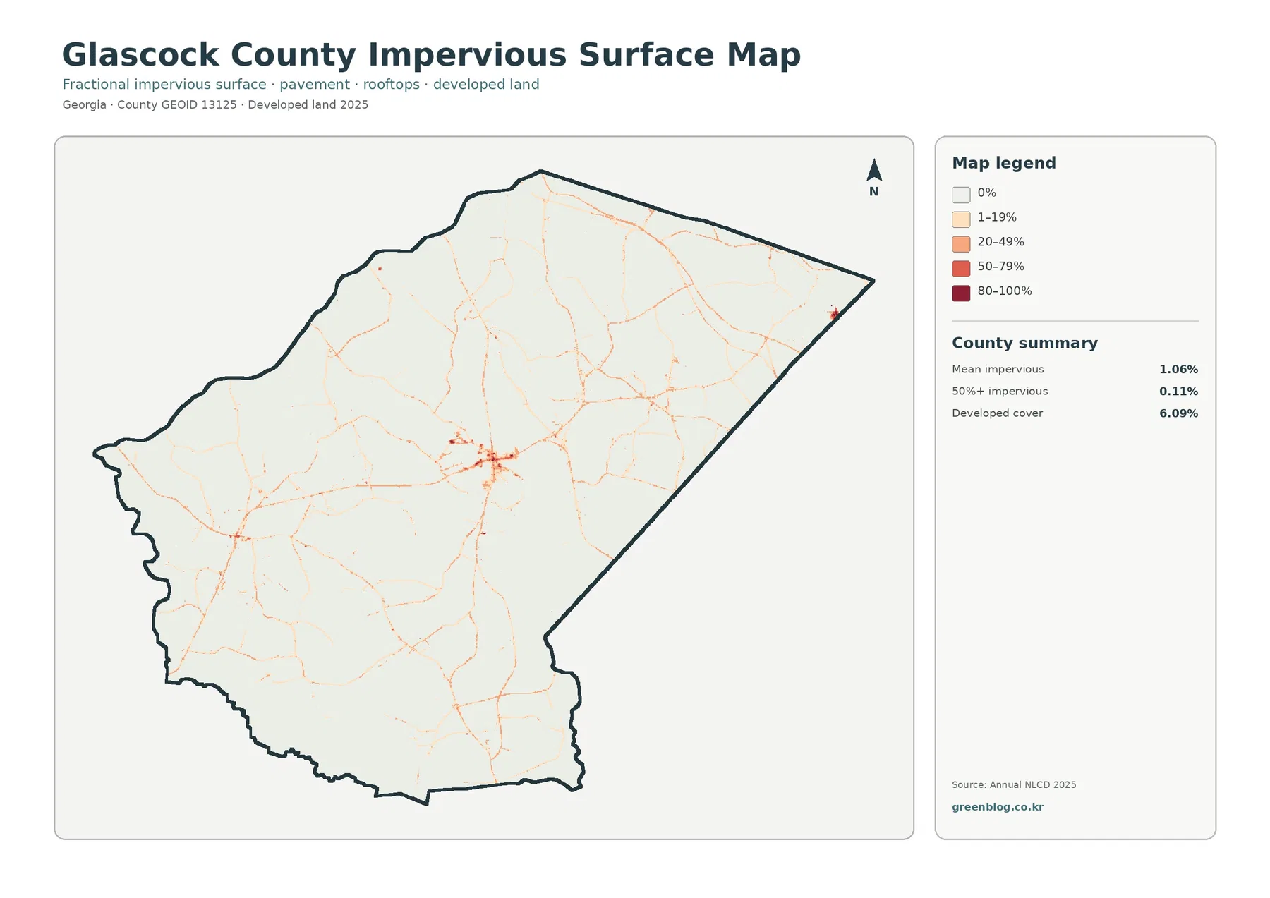
A small built core stands out in an otherwise low-impervious county
The impervious-surface view is one of the quickest ways to understand Glascock County’s development pattern. Most of the county remains in the lightest classes, and narrow lines trace the road network rather than broad urban districts. A stronger cluster appears near the center, where Gibson is located. The county’s official website places county government in Gibson, and Georgia’s community-planning material identifies Gibson at the intersection of State Routes 171 and 102, which provides useful context for the central concentration visible in the map.
Countywide mean imperviousness is only 1.06%, and land with at least 50% impervious cover accounts for 0.11%. Developed land is broader, at 6.09%, because a developed class can include yards, trees, soil, and other surfaces that still absorb water. That difference matters in a rural county. A neighborhood or roadside settlement may count as developed land without looking like a dense field of pavement and rooftops on the impervious map.
Outside the central cluster, hard surfaces mostly appear as thin road-linked traces and small isolated spots. There is also a compact dark mark near the northeastern edge and a few smaller points elsewhere, but none approach the size of the Gibson-area concentration. The map therefore supports a description of dispersed rural development with one clearer center, not a countywide urban footprint. Imperviousness should not be treated as a flood-risk score; drainage, soils, slope, rainfall, and stream conditions are separate factors.
The 2025 cover mix is more varied than the forest percentage suggests
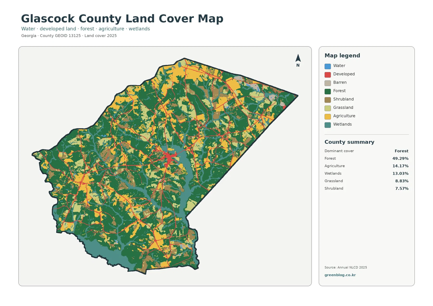
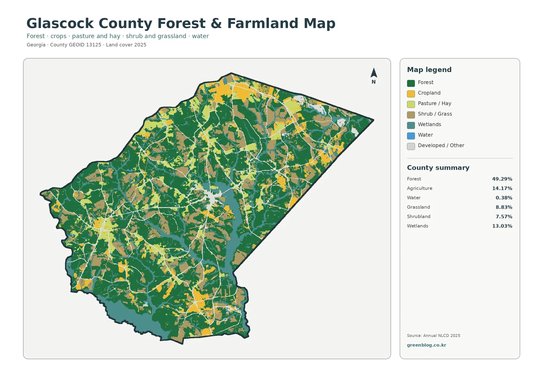
Forest leads the 2025 summary at 49.29%, but nearly half the county belongs to other cover types. Agriculture accounts for 14.17%, wetlands 13.03%, grassland 8.83%, and shrubland 7.57%. Water is a much smaller 0.38% in the forest-and-farmland summary. When these values are read together, Glascock County looks less like a uniformly wooded landscape and more like a changing mosaic of wooded blocks, working land, wet corridors, open ground, and small developed areas.
The general land-cover map makes that mosaic visible. Large forest blocks occupy much of the southwest, south-central interior, and several northern sections. Agricultural areas recur as yellow patches in the north, east, center, and south rather than forming one uninterrupted farming belt. Wetlands extend along the western boundary and into lower corridors farther south. Grassland and shrubland often sit between or beside the larger forest and agricultural patches, adding another layer of variation.
Land cover is not the same thing as zoning, ownership, or legal land use. It classifies what is physically covering the surface in the source data—such as forest, crop cover, wetland vegetation, water, or developed surfaces. A forest-colored cell is not automatically protected land, and an agriculture-colored cell is not automatically zoned for farming. Property decisions, permits, and parcel boundaries require the appropriate county or state records.
Forest and farmland form a patchwork rather than two separate zones
The simplified forest-and-farmland view is useful because it removes some of the visual competition among classes. Forest still forms the largest green blocks, while cropland and pasture or hay appear in repeated openings throughout the county. Those openings are especially noticeable across the northern half, in central sections around the road network, and in several eastern and southern pockets. They are not arranged as one broad agricultural plain.
Georgia’s Glascock County planning material describes farming and forestry as dominant sectors of the local economy. That local background is consistent with a map where both wooded land and agricultural cover occupy substantial space. The map should not be pushed beyond what it measures, however. It does not identify a crop variety, farm ownership, production value, or the current management of a particular field. Those questions require agricultural statistics or farm-level information.
Open cover also includes more than cropland. Grassland represents 8.83% and shrubland 7.57%, so many pale-green and brown areas are not simply “farms.” Some lie between wooded blocks, some border agricultural patches, and others form irregular openings of their own. Keeping those classes separate prevents a common reading error in which every non-forest, non-developed area is assumed to be agriculture.
Wetlands make the western edge an important reference point
The western boundary provides one of the clearest geographic anchors in the map set. Georgia community-planning material notes that the Ogeechee River forms part of Glascock County’s western boundary. On the land-cover maps, wetland colors follow much of that side of the county and continue into several southern and interior corridors. The relationship is useful for orientation, although the land-cover image is not a surveyed river or wetland-boundary map.
Wetlands cover 13.03% of the county, far more than the 0.38% mapped as open water in the simplified summary. That gap illustrates why water and wetland should not be combined when reading the legend. Open water represents visibly water-covered cells, while wetlands can include vegetated areas that remain saturated or seasonally wet. A county can therefore have a modest blue-water percentage and still contain extensive wetland cover.
The same planning document also identifies Rocky Comfort Creek as a local natural resource. The supplied land-cover image does not label individual streams, so it would be misleading to assign every wet corridor to a named creek. For watershed work, the land-cover map is best used as a broad surface-cover layer, then paired with a dedicated hydrography dataset when exact channels, drainage areas, or stream names are needed.
The 1985–2025 comparison has widespread class differences
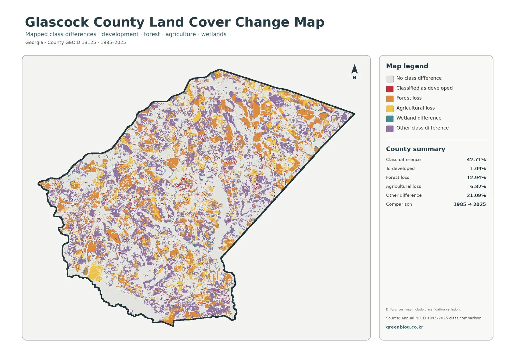
The change map looks much busier than the present-day maps. Class differences occupy 42.71% of the county in the comparison summary. Forest loss is listed at 12.94%, agricultural loss at 6.82%, change to developed at 1.09%, and other class difference at 21.09%. Orange, yellow, and purple areas appear across many parts of the county rather than forming a single change hotspot.
Forest-loss colors occur in sizable patches in northern, eastern, southwestern, and interior sections. Agricultural-loss colors are more scattered, while change-to-developed remains comparatively limited and is most noticeable around the central developed area and small road-linked locations. The numbers reinforce what the map suggests: only a small portion of the total class difference is labeled as a transition to developed land, so the widespread colored cells should not be described as broad urban expansion.
A class-difference map is not a direct construction or logging history. The map itself warns that classification variation may be included. Satellite observations from different years can classify edges, mixed vegetation, harvested or regrowing forest, narrow roads, and mixed pixels differently. A colored cell can represent real land-cover change, but it can also reflect the limits of comparing classified imagery across a long interval.
The comparison also gives only the two endpoints, 1985 and 2025. It cannot tell a reader exactly when a change occurred between those years. A place might have changed more than once, and a two-date comparison may not preserve that full sequence. Anyone investigating a specific parcel or event should use intermediate imagery, local records, or time-series data rather than treating this one map as a dated history of each cell.
How to read the four maps as one set
Start with a location, then switch maps without changing your point of reference. Around Gibson, the general map identifies a broader developed class, while the impervious view isolates the places with more pavement and rooftops. The forest-and-farmland map then simplifies the surrounding rural cover, making wooded and agricultural openings easier to compare. The change map answers a different question by marking where the 1985 and 2025 classifications differ.
Along the western boundary, the useful comparison changes. Wetlands and forest dominate the present-day cover view, while hard surfaces remain sparse on the impervious map. The change layer contains scattered differences in the same area, but those colors do not establish a wetland trend by themselves. A dedicated wetland inventory or hydrologic dataset would be needed to evaluate wetland gain, loss, or regulatory boundaries.
The northern and eastern agricultural patches offer another example. The simplified map makes fields and open cover easier to spot, but the full land-cover view is better when the surrounding shrubland, grassland, wetlands, and developed cells matter. Switching between the two prevents the legend from becoming an obstacle. A presentation can begin with the simpler view, then use the full map when the audience is ready for the additional classes.
Percentages summarize the county; pixels generalize the ground
County percentages are useful for comparison, but they do not explain where a class occurs or how it is shaped. Glascock County’s 13.03% wetland cover is divided among a long western band, southern corridors, and smaller interior pieces. Its 14.17% agriculture is also split among many patches. Two counties with the same percentage could look completely different if one has a single large block and the other has dozens of small fragments.
Annual NLCD is a raster product, meaning the landscape is represented by grid cells. Each cell receives a representative class, even when the ground within that cell contains more than one surface type. A narrow road beside trees, a small stream through forest, or a house surrounded by lawn can therefore be generalized. This is useful for consistent county-scale comparison, but it is not a substitute for a parcel survey, site plan, or high-resolution building map.
The 2025 label also matters. These maps describe the supplied 2025 classification rather than live conditions at the moment someone opens the page. Construction, timber harvest, regrowth, field rotation, or other changes after the observation and processing period may not be represented. For current site-specific work, recent aerial imagery and local records should be checked alongside the land-cover layer.
Useful ways to apply the maps without overreading them
For classroom work, Glascock County is a useful example of a rural landscape where forest is largest but not overwhelmingly dominant. Students can compare the 49.29% forest share with 14.17% agriculture and 13.03% wetlands, then locate where those classes actually occur. Adding the impervious map makes it possible to discuss why 6.09% developed land can coexist with only 1.06% mean imperviousness.
For watershed or environmental presentations, the western Ogeechee boundary and the wetland bands provide a clear place to begin. The central Gibson area can then be used as a contrast because hard surfaces are more concentrated there. This does not establish water quality, runoff volume, flood probability, or habitat condition. Those topics require hydrology, rainfall, soils, elevation, biological, or regulatory data in addition to land cover.
For local planning discussions, it is helpful to keep current cover and long-term class difference on separate slides. The 2025 layer answers what the surface is classified as now, while the 1985–2025 layer identifies where the two endpoint classifications differ. Mixing the two can lead an audience to confuse current acreage with change acreage. Clear map titles and dates are a simple way to prevent that mistake.
For reports and printed material, the downloadable JPG files are more convenient than the page previews. Each original is 2480×1754 pixels, and all four are packaged together. A user can select a single map for a short report or place matching maps side by side for comparison. The source size should be considered when choosing a large print format; the package does not claim that these files meet A3 at 300 dpi.
Frequently Asked Questions
What is the largest land-cover class in Glascock County?
Forest is the largest 2025 class at 49.29%. Agriculture follows at 14.17% and wetlands at 13.03%, with substantial grassland and shrubland as well. The map therefore shows a forest-led but highly mixed rural landscape rather than a county covered almost entirely by woods.
Why does the Gibson area look smaller on the impervious map than on the developed-land view?
Developed land can include lawns, trees, soil, and other permeable surfaces around homes, businesses, and roads. Imperviousness focuses on hard surfaces such as pavement and rooftops. Glascock County has 6.09% developed cover, but mean imperviousness is only 1.06% and the 50%+ impervious class covers 0.11%, so the darkest hard-surface footprint is much smaller.
Does the 42.71% class difference mean nearly half the county was physically transformed?
Not necessarily. The figure measures cells whose classifications differ between 1985 and 2025. Real forest, agricultural, and development changes can contribute, but classification variation and mixed pixels can also create differences. A site-specific history requires intermediate imagery or local records.
Sources and reference material
- MRLC Annual NLCD Data – official access and background for the land-cover data used for annual comparisons.
- USGS Annual NLCD Land Cover Classification – official definitions for forest, developed, agriculture, wetlands, and related land-cover classes.
- U.S. Census Bureau TIGER/Line Shapefiles – official geographic boundary resources used for county mapping.
- Glascock County official website – county government information and official Gibson contact location.
- Georgia DCA – Glascock County & Cities Plan Update – local context for Gibson, Mitchell, Edge Hill, the Ogeechee River, Rocky Comfort Creek, farming, and forestry.
Map File Information
The four original JPG maps used for this Glascock County land-cover set are provided together in one ZIP file.
- Included Versions: overall land cover, forest and farmland, impervious/developed land, and 1985–2025 land-cover change
- Printable Size: 2480×1754 pixels each
- File Type: four JPG images in one ZIP archive
Related Maps
- Appling County Georgia Land Cover Map
- Atkinson County Georgia Land Cover Map
- Bacon County Georgia Land Cover Map
Green Map creates custom-edited map images using open geographic data sources such as geoBoundaries, Natural Earth, OpenStreetMap, and government open data. These maps are edited visual materials, not raw data files, and are provided for education, documents, presentations, and graphic reference.