The 2023 state data for industrial-sector energy-efficiency programs show a highly uneven distribution of expected life-cycle program costs. In the U.S. Energy Information Administration (EIA) State Electricity Profiles, the 50 states plus the District of Columbia sum to $163.344 million for the combination Industrial + Expected Life Cycle of Programs + All Other Costs. California is highest at $25.589 million, followed by Oregon at $16.950 million and Michigan at $16.135 million. Those numbers are not industrial electricity bills, fuel expenditures, or the total cost of operating factories. They belong to a specific EIA-861 program-cost reporting framework.
EIA separates energy-efficiency program costs into customer incentives and all other costs. Customer incentives cover the financial value directly provided to participating customers, such as cash payments, favorable tariff treatment, in-kind design services, or other direct participation benefits. The measure used here is the other cost category. The time-period facet is also important: “Expected Life Cycle of Programs” represents life-cycle costs, which include the reporting-year incremental costs and anticipated future program costs. A state value should therefore not be read as a simple cash-outlay figure for calendar year 2023.
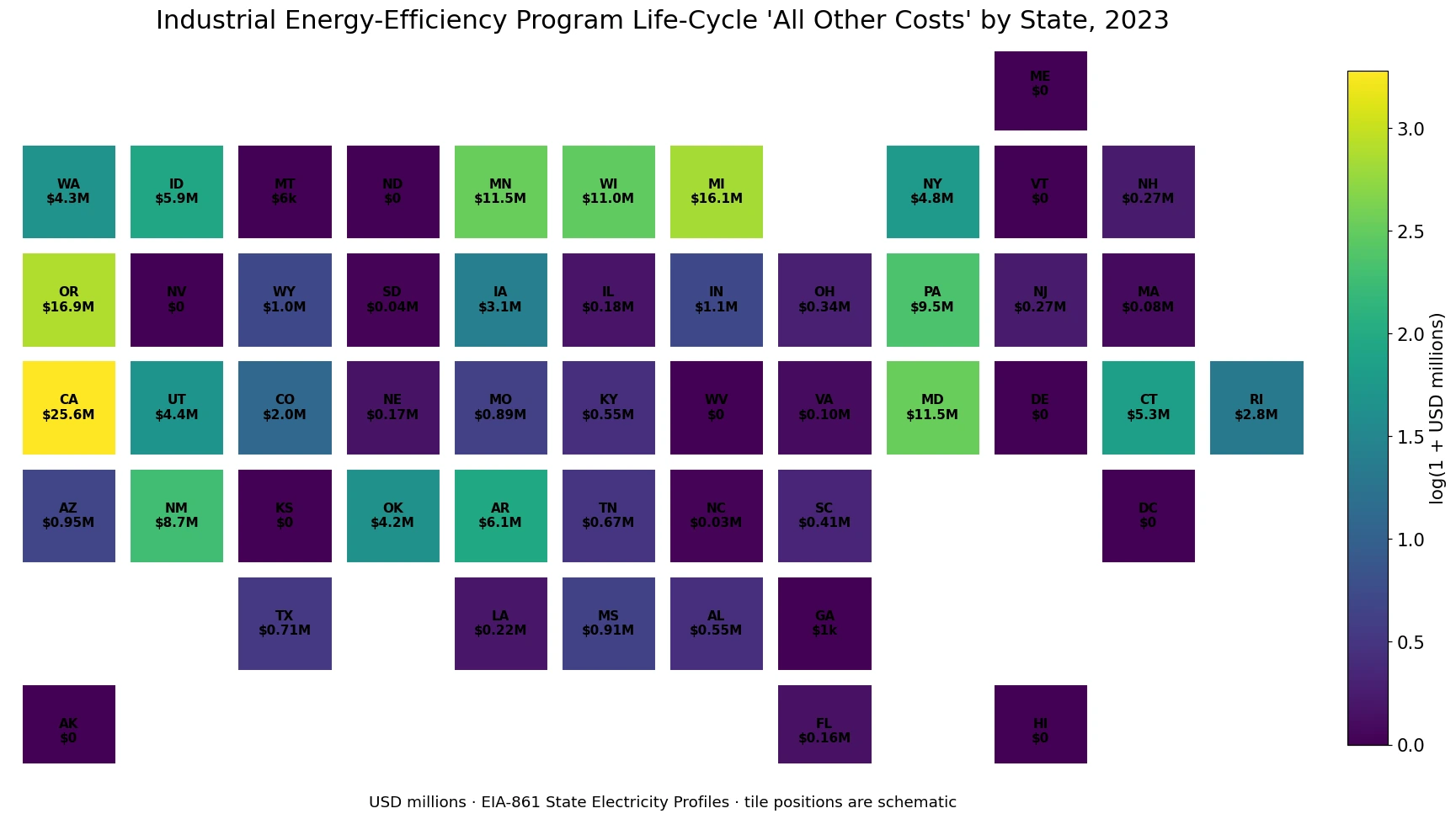
Table of Contents
California, Oregon, and Michigan form the leading group
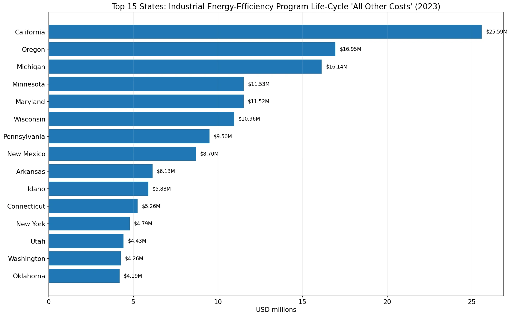
Sorting the 51 jurisdictions from highest to lowest puts California first at $25.589 million, Oregon second at $16.950 million, and Michigan third at $16.135 million. Together they account for $58.674 million, or 35.9% of the 51-row total. Minnesota and Maryland are nearly tied at $11.528 million and $11.523 million, while Wisconsin records $10.960 million. Pennsylvania at $9.504 million and New Mexico at $8.703 million also stand well above the median. The upper group spans the Pacific Coast, Great Lakes, Mid-Atlantic, Southwest, and South rather than forming one continuous region.
This ranking should not be converted into a league table of policy quality. Absolute program costs can reflect program scale, the number and size of participating industrial customers, the reporting entities operating in a state, expected program lives, and the mix of measures being funded. The supplied file does not contain program participation counts, industrial output, or savings per dollar. What it supports directly is a comparison of reported cost levels under one EIA definition, not a conclusion that a higher-cost state has a better or worse energy-efficiency program.
| Rank | State | Life-cycle all-other costs (USD millions) |
|---|---|---|
| 1 | California | 25.589 |
| 2 | Oregon | 16.950 |
| 3 | Michigan | 16.135 |
| 4 | Minnesota | 11.528 |
| 5 | Maryland | 11.523 |
| 6 | Wisconsin | 10.960 |
| 7 | Pennsylvania | 9.504 |
| 8 | New Mexico | 8.703 |
| 9 | Arkansas | 6.135 |
| 10 | Idaho | 5.885 |
| 11 | Connecticut | 5.263 |
| 12 | New York | 4.787 |
| 13 | Utah | 4.429 |
| 14 | Washington | 4.262 |
| 15 | Oklahoma | 4.193 |
The top five account for half of the total and the top ten for 75.2%
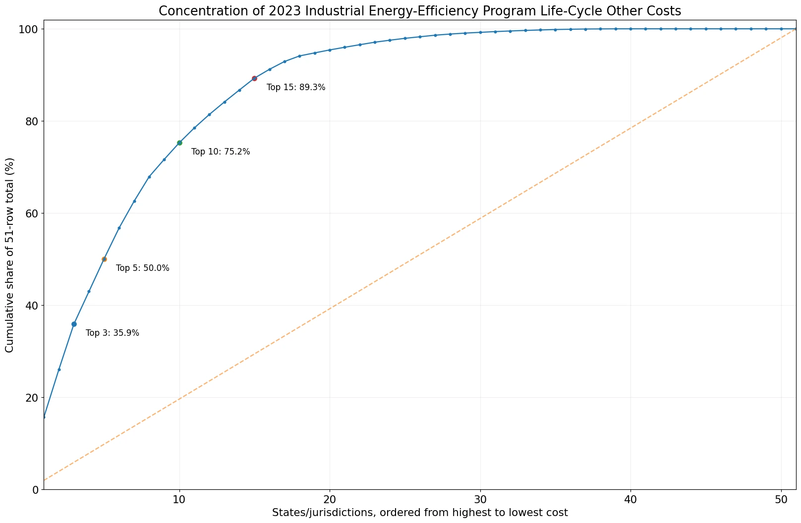
The distribution is strongly concentrated. The top five states sum to $81.725 million, equivalent to 50.0% of the 51-jurisdiction total. Expanding the group to the top ten raises the cumulative amount to $122.912 million and the share to 75.2%. The top fifteen account for 89.3%. Put differently, fewer than one-fifth of the jurisdictions account for roughly three-quarters of the reported life-cycle all-other costs in this industrial-sector slice.
That concentration also explains why the arithmetic mean is not a good description of a typical observation. The simple mean is $3.203 million, but the median is only $0.554 million. The first quartile is $0.033 million and the third quartile is $4.346 million. A statement such as “the average state reports about $3.2 million” is mathematically correct, yet it can hide how many jurisdictions are far below that level and how much the largest observations pull up the mean. Median, quartiles, and cumulative shares give a more faithful picture of the shape.
Ten reported zeros are numeric observations, not missing records
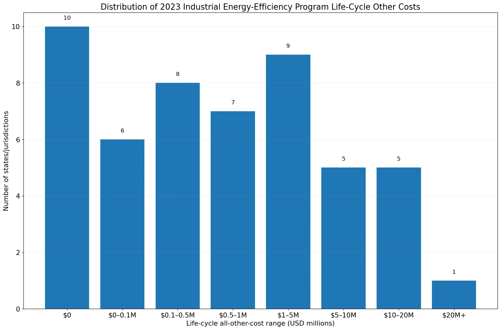
Alaska, the District of Columbia, Delaware, Hawaii, Kansas, Maine, North Dakota, Nevada, Vermont, and West Virginia have a reported value of zero for this exact metric slice. All 51 rows contain numeric observations, so the file has no missing state value to impute. The zeroes are therefore preserved as zeroes in the statistics and graphics. At the same time, a zero in this field should not be interpreted as proof that a state had no energy-efficiency activity. The observation refers to one sector, one cost category, and one life-cycle reporting definition; other sectors or cost fields may still have nonzero values.
The lower end of the distribution is broad. Ten jurisdictions are at zero, six are above zero but no more than $0.1 million, eight are above $0.1 million and no more than $0.5 million, and seven are above $0.5 million and no more than $1 million. Together, 31 of 51 jurisdictions, or 60.8%, are at or below $1 million. Only eleven exceed $5 million, and California is the only observation above $20 million. This combination of many small values and a short upper tail of large values produces the large mean-median gap.
Life-cycle cost is not the same as reporting-year cost
Form EIA-861 distinguishes reporting-year incremental costs from incremental life-cycle costs. Reporting-year incremental costs are associated with the incremental savings reported for the year, while life-cycle costs include anticipated program costs over the expected life of the savings. EIA instructions also state that startup costs incurred in earlier years may be included when they are part of the program supporting the incremental year, and that reporting-year and life-cycle costs can sometimes be equal when most expenditures occur in the first year. The distinction is essential when interpreting a state map.
A large life-cycle value therefore does not mean the same amount was paid out during 2023. Likewise, a small life-cycle value does not automatically imply little future activity. Budget execution, utility revenue requirements, customer bills, and annual cash spending answer different questions and require different data. The safest interpretation is narrower: the chart compares the expected life-cycle amount reported in the “all other costs” category for industrial energy-efficiency programs.
Customer incentives are a separate cost category
The EIA framework is designed to keep direct customer benefits separate from the rest of program costs. That means a high all-other-cost value does not tell us how much money industrial participants received as rebates or other direct incentives. A state could have high customer incentives and relatively modest other costs, or the reverse. Combining the two categories can provide a broader view of total program cost, but the two components should remain identifiable because they describe different flows of program resources.
The cost data are also separate from energy savings. EIA publishes life-cycle energy savings in MWh and peak-demand savings in MW in the same broader table family. A cost-effectiveness measure such as dollars per MWh would require a carefully matched savings series using the same sector and period definition. It cannot be calculated responsibly from this one cost field alone. The current article therefore avoids inventing a savings denominator or interpreting high costs as either efficient or inefficient without the matching outcome data.
The national annual table is close to, but not identical with, the 51-row sum
EIA’s Electric Power Annual Table 10.2 reports $163.528 million for 2023 industrial “Life Cycle Costs – All Other Costs.” The 51 state-and-D.C. observations in the State Electricity Profiles sum to $163.344 million. The difference is $0.184 million, about 0.11% of the national table value. The two figures are close enough to provide a useful magnitude cross-check, but they should not be forced into arithmetic identity. The supplied state file does not document the exact reason for the small difference between the two EIA presentations.
All rankings and distribution statistics in this article are therefore calculated only from the internally consistent 51-row state dataset. The national table is used as a separate reference point. This approach avoids mixing tables that may differ slightly in revision timing or aggregation conventions. When multiple official tables cover a similar concept, matching the field definition and the aggregation basis is more important than assuming every published total must reproduce the sum of a different presentation exactly.
The geography is descriptive, not causal
The upper observations are geographically diverse: California and Oregon are on the Pacific Coast; Michigan, Minnesota, and Wisconsin are in the Great Lakes and Upper Midwest; Maryland and Pennsylvania are in the Mid-Atlantic; New Mexico is in the Southwest; and Arkansas and Idaho also enter the top ten. Zero and very small observations are similarly scattered across regions. The pattern shows that reported costs vary sharply by state, but it does not identify the reason for that variation.
Explaining the differences would require additional variables such as industrial electricity sales, the number of industrial customers, program participation, measured energy savings, incentive payments, the number of reporting utilities or administrators, and industrial output. Absolute cost is especially sensitive to scale. A follow-up analysis could normalize costs by industrial electricity sales or participant counts, but those would be new derived indicators and should be labeled as such rather than presented as values published directly by EIA.
What this metric can and cannot answer
The data can answer where the reported industrial-sector expected life-cycle all-other costs were largest in 2023, how concentrated the 51 values were, and how many states reported low or zero values. It can also support a clean state comparison because every row shares the same year, unit, sector, cost field, and period facet. It cannot by itself answer which state saved the most electricity, which program was most cost-effective, how much industrial customers paid on their bills, or how much utilities spent in cash during 2023.
It also should not be confused with industrial energy expenditures from EIA’s State Energy Data System. Those expenditures describe money spent on energy products and electricity by the industrial sector. This dataset instead concerns costs of energy-efficiency programs reported through Form EIA-861. Similar words such as “industrial costs” can refer to very different accounting boundaries, so preserving the program context in the title and first paragraphs is important for both search clarity and statistical accuracy.
Data source and calculation method
The statistical source is the U.S. Energy Information Administration’s State Electricity Profiles – Costs and Savings from Energy Efficiency Programs, based on Form EIA-861. The selected observation slice is year 2023, Industrial sector, Expected Life Cycle of Programs, and All Other Costs. The source unit is thousand dollars. Display values are converted to USD millions by dividing by 1,000; rankings and shares are calculated from the original thousand-dollar observations.
The file contains 51 unique state or jurisdiction codes covering the 50 states and the District of Columbia. All observations are dated 2023, all 51 have numeric values, ten are exactly zero, and none are missing. The 51-row sum is $163.344 million, the mean is $3.203 million, and the median is $0.554 million. The representative tile graphic joins every state code exactly once. Its tile layout is schematic rather than an administrative-boundary map, and no missing value was replaced with zero or borrowed from another year.
Frequently Asked Questions
Which state had the highest 2023 industrial energy-efficiency program life-cycle all-other costs?
California was highest at $25.589 million, followed by Oregon at $16.950 million and Michigan at $16.135 million.
Does “All Other Costs” mean industrial energy bills or electricity expenditures?
No. It is an EIA-861 energy-efficiency program cost category reported separately from direct customer incentives.
Does “Expected Life Cycle of Programs” mean only cash spent during 2023?
No. Life-cycle costs include reporting-year incremental costs and anticipated future program costs, so the measure is broader than a one-year cash expenditure.
Do the ten zero values mean those states had no energy-efficiency programs?
Not necessarily. Zero is the reported value for this exact industrial-sector, life-cycle, all-other-cost field; other sectors or cost categories may still be nonzero.
Related Maps
Green Map creates custom-edited map images using open geographic data sources such as geoBoundaries, Natural Earth, OpenStreetMap, and government open data.
These maps are edited visual materials, not raw data files, and are provided for education, documents, presentations, and graphic reference.