The U.S. Energy Information Administration reports a 2024 annual average kerosene price for all end-use sectors in every state and the District of Columbia. The common unit is dollars per million Btu, which makes the 51 jurisdictions directly comparable on the same energy-content basis. The values range from $19.46 per million Btu in Texas to $30.39 in Michigan. That is a difference of $10.93 per million Btu between the lowest and highest observations. Because every row uses the same year, unit, metric and geographic level, the comparison does not mix time periods or fill missing values.
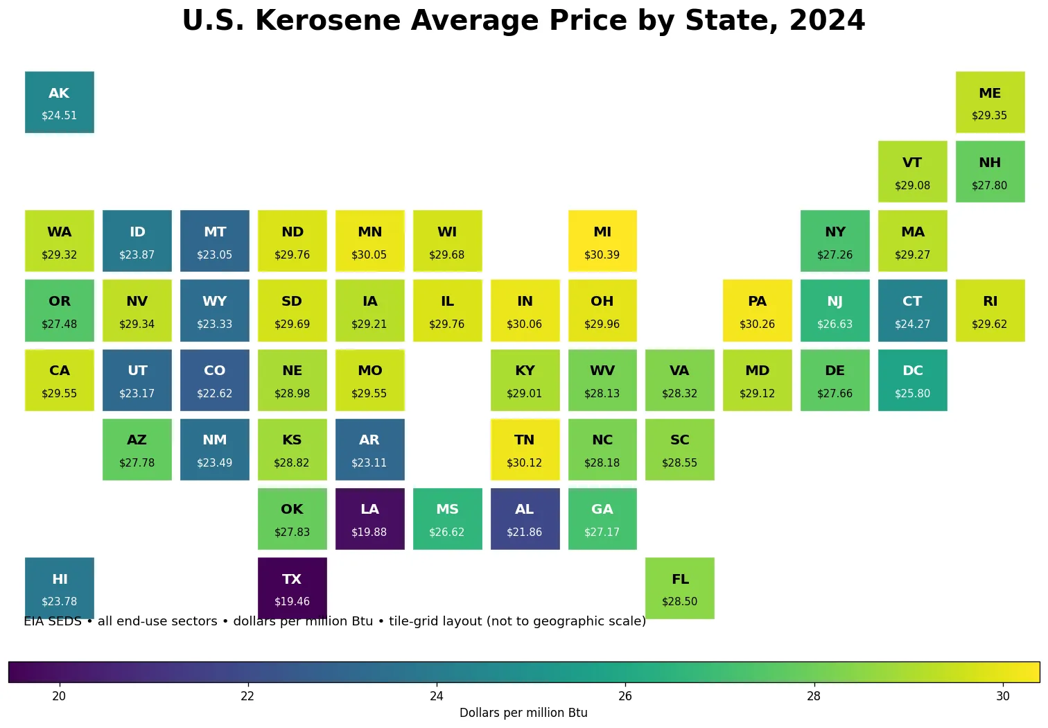
Table of Contents
What the EIA kerosene price measure means
This series should be read as an energy-price statistic, not as a posted retail price per gallon. EIA identifies the metric as kerosene average price, all end-use sectors and publishes it in dollars per million Btu. Using an energy-content unit is important because it expresses the price relative to the amount of energy represented, rather than the physical volume of fuel alone. The phrase “all end-use sectors” also matters: the observation is not labeled as a residential-only, commercial-only or industrial-only price. It is the state-level annual value for the combined end-use scope specified by the SEDS series.
The source provides one fixed 2024 observation for each jurisdiction, with no imputation or aggregation added here. That means the most defensible comparisons are descriptive: which jurisdictions have higher or lower reported prices, how tightly the middle of the distribution is grouped, and where unusually low or high values appear. The data do not identify the reason for a state’s position. Transportation costs, fuel-market structure, taxes, supply chains, customer composition and many other factors could matter, but those possible explanations are not contained in this one series and should not be inferred from the price values alone.
Michigan had the highest 2024 value, while Texas had the lowest
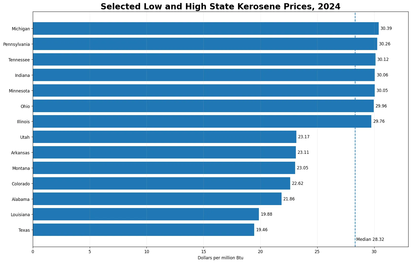
Michigan recorded the highest value at $30.39 per million Btu. Pennsylvania followed at $30.26, Tennessee at $30.12, Indiana at $30.06 and Minnesota at $30.05. The top five are therefore packed into a narrow $0.34 range, even though they come from different parts of the country. Ohio, North Dakota, Illinois, South Dakota and Wisconsin also sit close to the top, all between $29.68 and $29.96. The upper end is consequently not defined by one isolated state; it contains a cluster of jurisdictions near the $30 mark.
At the other end, Texas was lowest at $19.46 per million Btu, followed by Louisiana at $19.88. Alabama was $21.86, Colorado $22.62 and Montana $23.05. Arkansas, Utah, Wyoming, New Mexico and Hawaii also fall in the lower portion of the distribution. The gap between Texas and Michigan is $10.93 per million Btu, and Michigan’s value is about 1.56 times Texas’s. Those figures describe the size of the observed spread; they do not show that consumers in one state necessarily paid 56% more for every kerosene transaction, because the underlying statistic is an annual average across the specified end-use scope.
| Jurisdiction | 2024 price (dollars per million Btu) |
|---|---|
| Michigan | $30.39 |
| Pennsylvania | $30.26 |
| Tennessee | $30.12 |
| Indiana | $30.06 |
| Minnesota | $30.05 |
| Texas | $19.46 |
| Louisiana | $19.88 |
| Alabama | $21.86 |
| Colorado | $22.62 |
| Montana | $23.05 |
Most jurisdictions are closer to the upper 20s than the extremes
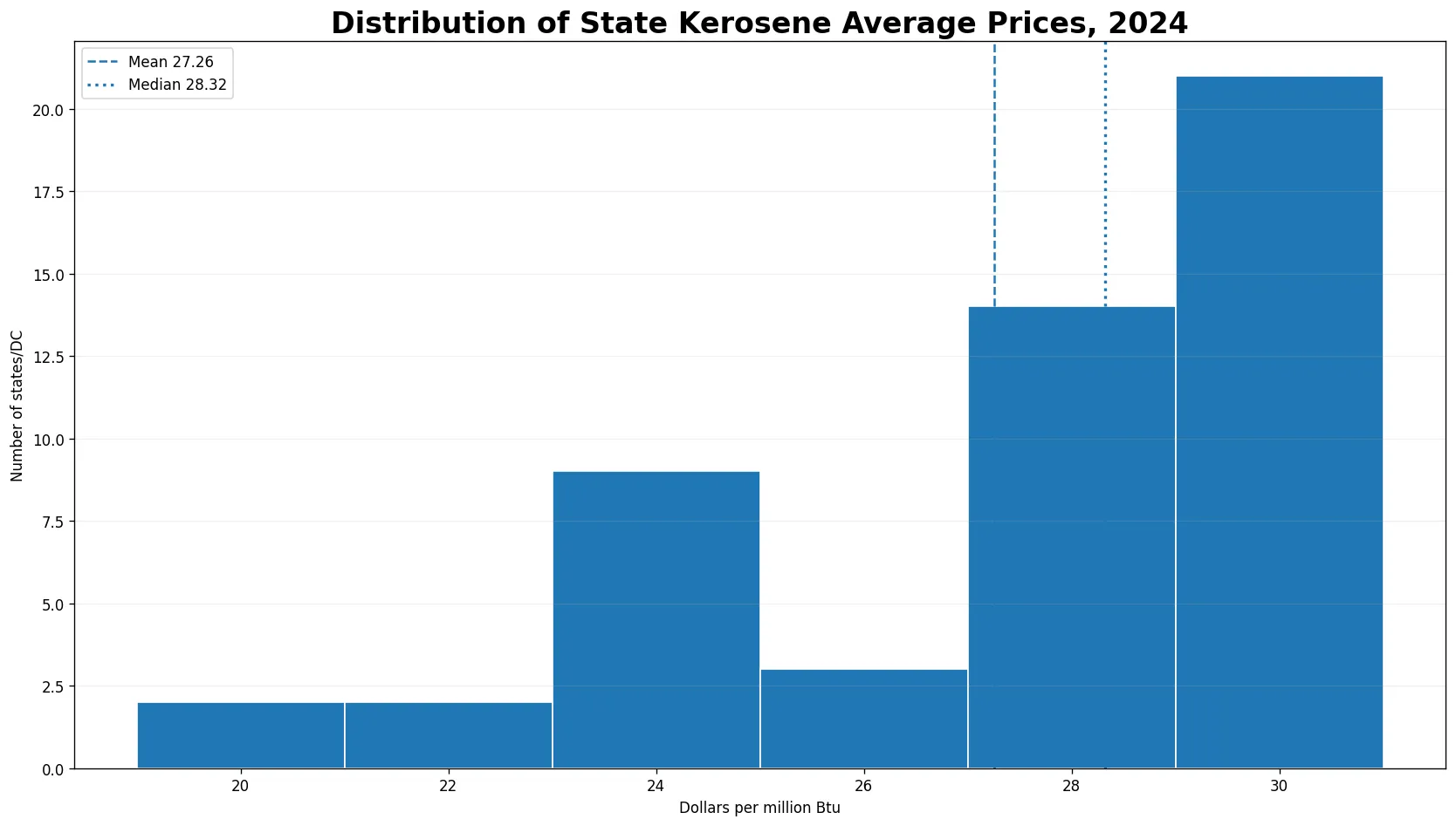
The distribution is more concentrated than the full minimum-to-maximum range might suggest. The arithmetic mean across the 51 jurisdictions is $27.26 per million Btu and the median is $28.32. The first quartile is about $25.16 and the third quartile about $29.45, so the middle half of observations fits inside a band only about $4.30 wide. The 10th percentile is $23.11 and the 90th percentile is $29.96. In other words, the central part of the dataset is much tighter than the roughly $11 spread created by the lowest and highest states.
Using simple price bands makes the pattern easier to see. Eleven jurisdictions are below $24 per million Btu. Five are between $24 and $26.99. Fourteen fall from $27 through $28.99, sixteen are between $29 and $29.99, and five reach $30 or more. Taken together, 30 of the 51 jurisdictions fall from $27 up to but not including $30. Another 21 are at $29 or above. This concentration explains why a map with a single broad color scale can make many states look similar even when their values differ by several tenths of a dollar per million Btu.
What the tile-grid map adds to the comparison
The tile-grid map is designed for a fast spatial read while keeping every jurisdiction visible, including Alaska, Hawaii and the District of Columbia. It is intentionally not a conventional area-weighted choropleth. A large state therefore does not occupy more visual space than a small one, which prevents geography alone from dominating the display. Each tile contains the exact state abbreviation and rounded price, while the color scale provides an immediate high-to-low cue. All 51 data rows match a tile, so there are no unplotted jurisdictions and no missing prices represented as zero.
Several neighboring or nearby jurisdictions differ noticeably. Texas at $19.46 is far below Oklahoma at $27.83 and New Mexico at $23.49. Louisiana at $19.88 is also below Mississippi at $26.62 and Arkansas at $23.11. In the Great Lakes area, Michigan at $30.39, Indiana at $30.06, Ohio at $29.96, Illinois at $29.76 and Wisconsin at $29.68 form a set of relatively high observations. These are descriptive geographic patterns only. A map can reveal adjacency and clustering, but the price series itself cannot establish the market or policy mechanisms behind those patterns.
How to interpret a state ranking without overstating it
A rank is useful for locating a state within this particular 2024 series, but the exact position should not be treated as a permanent characteristic. Many values are close together. For example, Indiana at $30.06 and Minnesota at $30.05 differ by only one cent per million Btu, while North Dakota and Illinois both report $29.76. Small differences of this kind can change ordering without representing a large economic gap. For practical interpretation, price bands, the median and the overall spread are often more informative than emphasizing every ordinal rank.
It is also important to preserve the unit when comparing this series with other fuel statistics. A kerosene price expressed in dollars per million Btu is not directly interchangeable with a price per gallon, a total expenditure value, total fuel consumption, or an average heat-content measure. Those metrics answer different questions. A state could have a high energy-normalized price but low kerosene consumption, or a lower price but greater use. To understand the state energy market, price should therefore be viewed alongside consumption, heat content and sector-specific data rather than used as a stand-alone measure of market size.
Why the 2024 common year improves comparability
One strength of this dataset is that every jurisdiction uses 2024. Cross-state comparisons can become misleading when one state’s latest observation is recent and another’s is several years old, especially for energy prices that can move over time. That problem is absent here: the 50 states and District of Columbia all share the same annual reference year. The data also use the same unit and series definition across rows. Those conditions support direct descriptive comparison of levels in 2024, while still leaving open the separate question of how each state changed from earlier years.
This article does not calculate a trend because only the verified 2024 state slice is used. A trend statement such as “prices rose” or “prices fell” would require the corresponding earlier annual observations from the same series. Likewise, the 2024 cross section cannot tell whether the difference between Michigan and Texas widened or narrowed over time. Keeping those questions separate prevents a snapshot from being mistaken for a time series. The current evidence supports a clear statement about the 2024 distribution, not an unsupported claim about direction or cause.
Practical takeaways from the 51-jurisdiction comparison
The central result is straightforward. U.S. state-level kerosene average prices in this EIA all-end-use series were mostly in the upper $20s per million Btu in 2024, but the full range was wider. Michigan was highest at $30.39 and Texas lowest at $19.46. The median of $28.32 sits above the mean of $27.26 because several low observations pull the average downward. The middle half of jurisdictions falls between roughly $25.16 and $29.45, while only five reach $30 or more. These figures provide a compact benchmark for comparing any individual state with the national state-level distribution.
For a visitor looking up one state, the best reading sequence is to note the state’s exact value on the map, compare it with the median, and then see whether it sits in the central cluster or near an extreme. For research use, keep the EIA series identity, year and unit attached to the number. The official source is the U.S. Energy Information Administration’s State Energy Data System (SEDS). Because the values are annual state observations for a specific metric, they can be combined responsibly with other EIA state indicators only when the metric definitions, units and years are aligned.
Source: U.S. Energy Information Administration, State Energy Data System (SEDS). Metric: Kerosene average price, all end-use sectors. Year: 2024. Unit: dollars per million Btu. Coverage: 50 U.S. states and the District of Columbia.
Frequently Asked Questions
Which jurisdiction had the highest kerosene average price in 2024?
Michigan had the highest value in the EIA SEDS state series at $30.39 per million Btu.
Which jurisdiction was lowest, and what was the median?
Texas was lowest at $19.46 per million Btu. The median across the 50 states and Washington, D.C. was $28.32.
Is this the same as a retail kerosene price per gallon?
No. The EIA series is an annual all-end-use average expressed in dollars per million Btu, not a specific retail price per gallon.
Related Articles
Green Map creates custom-edited map images using open geographic data sources such as geoBoundaries, Natural Earth, OpenStreetMap, and government open data. These maps are edited visual materials, not raw data files, and are provided for education, documents, presentations, and graphic reference.