The U.S. County Household Income Map shows a country with wide local differences rather than one smooth national income gradient. Among county-level records that pass the supplied reliability rule, the midpoint of the county estimates is $65,714. Loudoun County, Virginia sits at the top at $181,765, while Owsley County, Kentucky is the lowest reliable estimate at $22,188. The more useful story, however, is geographic: high-income counties often connect into broad multi-county zones, lower-income counties form long bands across parts of Appalachia and the South, and some of the largest gaps occur between counties that share a border.
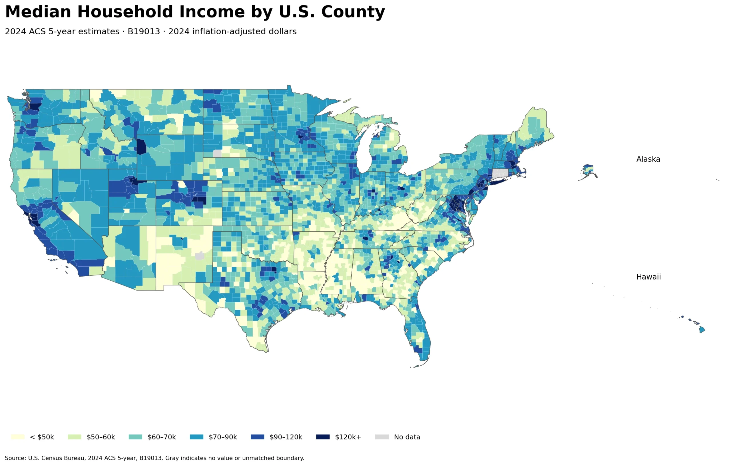
Table of Contents
What the U.S. County Household Income Map actually measures
The values come from the U.S. Census Bureau American Community Survey table B19013, which reports median household income in the past 12 months. Median is the midpoint of the household-income distribution within each county: half of households are above the estimate and half are below it. It is not an average, and it should not be read as disposable income, wealth, individual earnings, or purchasing power after local housing costs. That distinction matters because a county with a high dollar income can also have high living costs.
For the 3,135 county-level records eligible for ranking, the 25th percentile is $56,745, the median county estimate is $65,714, and the 75th percentile is $75,848. The bottom-decile cutoff is about $49,079, while the top-decile cutoff is about $89,423. These are percentiles across county estimates, not the median income of all U.S. households. A small rural county counts once, just as a very populous county counts once, so the figures describe the geography of counties rather than a population-weighted national household statistic.
The top end is spread across several strong regional clusters
Loudoun County leads the reliable estimates at $181,765. Santa Clara and San Mateo counties in California follow, and Fairfax County, Virginia and Howard County, Maryland round out the first five. The top ten also include Douglas County, Colorado; Marin County, California; Los Alamos County, New Mexico; Nassau County, New York; and Forsyth County, Georgia. That list already makes an important point: the highest county incomes are not confined to one state or one coast.
| Rank | County-level geography | Median household income | MOE |
|---|---|---|---|
| 1 | Loudoun County, Virginia | $181,765 | ±$3,438 |
| 2 | Santa Clara County, California | $164,281 | ±$1,955 |
| 3 | San Mateo County, California | $158,855 | ±$2,851 |
| 4 | Fairfax County, Virginia | $153,637 | ±$1,635 |
| 5 | Howard County, Maryland | $149,763 | ±$3,158 |
| 6 | Douglas County, Colorado | $149,594 | ±$2,519 |
| 7 | Marin County, California | $149,091 | ±$4,474 |
| 8 | Los Alamos County, New Mexico | $147,139 | ±$10,556 |
| 9 | Nassau County, New York | $146,202 | ±$1,472 |
| 10 | Forsyth County, Georgia | $143,784 | ±$2,813 |
When counties at or above the top-decile threshold of roughly $89,423 are grouped by shared borders, Virginia contains a connected component of 28 counties and independent cities. California has a connected high-income component of 27 counties, Colorado has one of 20, New Jersey has one of 13, and Maryland has one of 12. The map therefore looks less like a handful of isolated dark spots and more like several regional systems where neighboring counties repeatedly fall into the upper tenth of the national county distribution.
Low-income counties form long connected bands, not just isolated outliers
The lowest reliable estimate is Owsley County, Kentucky at $22,188. Randolph County, Georgia and Lake County, Tennessee are next, followed by Greene County, Alabama and Wolfe County, Kentucky. The raw difference between the highest and lowest reliable county estimates is $159,577; the top value is about 8.2 times the bottom value. That ratio is useful as a scale check, but it is not a direct measure of household inequality because county living costs, household composition, and other local conditions are not included.
| Rank | County-level geography | Median household income | MOE |
|---|---|---|---|
| 1 | Owsley County, Kentucky | $22,188 | ±$9,297 |
| 2 | Randolph County, Georgia | $28,380 | ±$13,486 |
| 3 | Lake County, Tennessee | $28,814 | ±$6,937 |
| 4 | Greene County, Alabama | $29,200 | ±$5,134 |
| 5 | Wolfe County, Kentucky | $30,417 | ±$10,309 |
| 6 | Bullock County, Alabama | $31,310 | ±$9,971 |
| 7 | Bell County, Kentucky | $31,354 | ±$3,340 |
| 8 | McDowell County, West Virginia | $31,559 | ±$2,515 |
| 9 | Claiborne County, Mississippi | $31,897 | ±$7,278 |
| 10 | Allendale County, South Carolina | $32,328 | ±$7,995 |
Using the bottom-decile cutoff of about $49,079, the largest connected low-income component in the map contains 54 counties or county equivalents across parts of Louisiana, Arkansas, and Mississippi. Another component of 37 runs through parts of Kentucky and Tennessee. Mississippi also contains a 21-county connected group, Alabama a 19-county group, and Georgia a 15-county group. This is why a county map adds information that a state ranking cannot: it shows where a low value continues across borders and where the pattern breaks.
Some of the sharpest differences are between neighbors
Shared borders do not guarantee similar household incomes. Santa Clara County, California is estimated at $164,281, while neighboring Merced County is $65,510, a gap of $98,771. Los Alamos County, New Mexico is $147,139 next to Rio Arriba County at $57,155, a difference of $89,984. In New York, the Bronx is $48,676 and adjacent Westchester County is $118,976, a $70,300 gap. These examples are more informative than a simple state average because they identify exact places where the income surface changes abruptly.
The map does not tell us what caused those gaps. Industry mix, commuting patterns, educational attainment, housing costs, age structure, and many other variables could matter, but none of those should be inferred from B19013 alone. A neighboring-county contrast is best treated as a question generator: it identifies a place where additional data may be worth examining, rather than proving a causal explanation.
How wide is the county distribution?
Roughly one quarter of reliable county estimates are below $56,745, and one quarter are above $75,848. The distance between those two quartiles is $19,102. Moving from the 10th-percentile cutoff to the 90th-percentile cutoff adds about $40,344. Those broad percentile gaps help explain why the national map has large areas in different color bands even before the most extreme counties are considered.
Reliability matters, especially for small counties
The ACS table contains 3,143 county-level income values. For ranking, this analysis keeps 3,135 estimates with a coefficient of variation (CV) of 0.30 or less. Eight records have higher relative uncertainty and are excluded from the ranking tables, while De Baca County, New Mexico has no source value. Those caution records are not used in the top or bottom ranking tables. A small number of current county-equivalent codes also do not line up with the boundary layer used for the visualization, so a few map areas may appear gray even though the numeric analysis uses the current ACS records.
Margins of error are especially important near the bottom of the ranking. Owsley County’s estimate is $22,188 with a margin of error of ±$9,297, while Loudoun County’s $181,765 estimate has a margin of error of ±$3,438. The enormous gap between those two counties is still clear, but very close rankings should not be treated as precise league-table positions when their uncertainty intervals overlap.
How to use the map without overreading it
- The 2024 ACS 5-year estimate is a 60-month period estimate based on data collected from 2020 through 2024, not a one-year snapshot.
- B19013 is reported in 2024 inflation-adjusted dollars.
- Median household income is not the same as cost-of-living-adjusted purchasing power or household wealth.
- Connected high- or low-income county clusters describe geography and adjacency; they do not identify the cause of the pattern.
- Use margins of error when comparing counties with similar estimates, especially small-population areas.
Data source and calculation notes
The income estimate is from the U.S. Census Bureau 2024 ACS 5-year table B19013. B19013_001E is the estimate for median household income in the past 12 months in 2024 inflation-adjusted dollars, and B19013_001M is its margin of error. Rankings use only county-level estimates with a coefficient of variation (CV) of 0.30 or less.
Percentiles are calculated across reliable county estimates with each county receiving equal weight. Spatial clusters are constructed by applying the top- or bottom-decile threshold and then connecting counties that share a boundary. This is an original geographic grouping for the map analysis; it is not a Census metropolitan-area classification and it is not population weighted.
Frequently asked questions
What does median household income mean?
It is the midpoint of the household-income distribution: half of households are above the estimate and half are below it. It is not the same as average household income, which can be pulled upward by a relatively small number of very high-income households.
Does the 2024 ACS 5-year estimate describe only calendar year 2024?
No. ACS 5-year estimates pool 60 months of survey data. The 2024 ACS 5-year product uses data collected from 2020 through 2024, and B19013 reports the result in 2024 inflation-adjusted dollars.
Should the county rankings be treated as exact?
No. ACS values are survey estimates and include margins of error. The ranking tables here use only estimates with a coefficient of variation (CV) of 0.30 or less, but counties with similar estimates can still have overlapping uncertainty intervals and should not be over-ranked.
Related Articles
- U.S. County Mortgage Cost Burden Map – 2024 ACS Patterns
- U.S. County Severe Rent Burden Map – Where Rent Takes Half of Income
Green Map creates custom-edited map images using open geographic data sources such as geoBoundaries, Natural Earth, OpenStreetMap, and government open data. These maps are edited visual materials, not raw data files, and are provided for education, documents, presentations, and graphic reference.