U.S. County Median Home Value Map compares the Census Bureau’s 2024 ACS 5-year estimate for the median value of owner-occupied housing units across counties and county equivalents in the 50 states and the District of Columbia. The source table provides 3,144 geographic rows; 3,139 have a usable value for mapping. The national county pattern is highly uneven, so a map is more informative than a single U.S. average.
The measure is in U.S. dollars and comes directly from ACS table B25077. It is not a list of recorded home-sale prices, and it should not be read as a monthly real-estate market index. The value is most useful here because the same definition, geographic unit, and source year can be compared across thousands of counties.
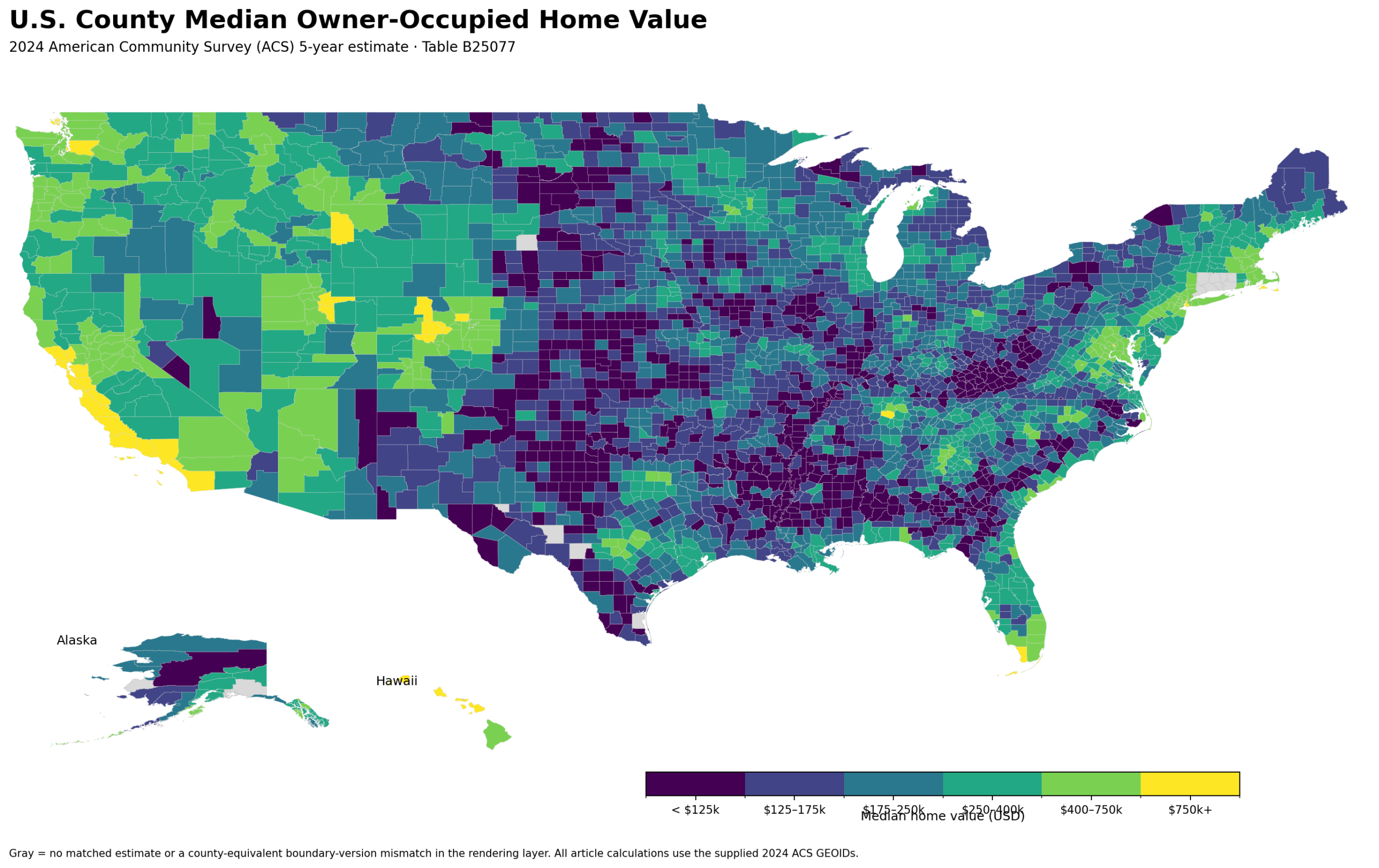
Table of Contents
What the 2024 county distribution looks like
Across the 3,139 counties with values, the median county estimate is $185,300. The first quartile is $141,450 and the third quartile is $269,500, meaning half of the county estimates fall between those two levels. The arithmetic mean is higher at $227,732, which reflects the long upper tail created by a relatively small number of very high-value counties.
That upper tail is substantial. 139 counties or county equivalents are at or above $500,000, 38 are at or above $750,000, and 13 exceed $1,000,000. At the other end, 892 are below $150,000. A county map makes this spread easier to see because high and low values are not distributed evenly across the country.
What “median home value” measures here
ACS table B25077 measures the median value of owner-occupied housing units. “Median” means the estimate at the middle of the local value distribution; it does not mean that most homes in the county are worth exactly that amount. It also does not cover renter-occupied units as a home-value measure.
This distinction matters when the map is compared with other housing statistics. A county can have a high median owner-occupied home value without having the highest rent burden, the fastest recent price growth, or the lowest affordability. Those questions use different numerators, denominators, or time comparisons and need their own data.
Counties above the national middle
Among rows approved for ranking, Teton County, Wyoming is highest at $1,633,900. Nantucket County, Massachusetts follows at $1,593,800, and San Mateo County, California is at $1,559,600. Marin and Santa Clara counties in California are also above $1,490,000. The concentration of several California counties near the top is a stronger spatial signal than one isolated extreme value.
| County | Median owner-occupied home value | 90% MOE |
|---|---|---|
| Teton County, Wyoming | $1,633,900 | ±$191,937 |
| Nantucket County, Massachusetts | $1,593,800 | ±$149,009 |
| San Mateo County, California | $1,559,600 | ±$16,159 |
| Marin County, California | $1,507,300 | ±$27,346 |
| Santa Clara County, California | $1,490,600 | ±$14,163 |
| San Francisco County, California | $1,394,500 | ±$20,642 |
| Dukes County, Massachusetts | $1,165,800 | ±$68,458 |
| Pitkin County, Colorado | $1,139,100 | ±$222,109 |
| New York County, New York | $1,090,500 | ±$28,044 |
| Alameda County, California | $1,090,100 | ±$6,313 |
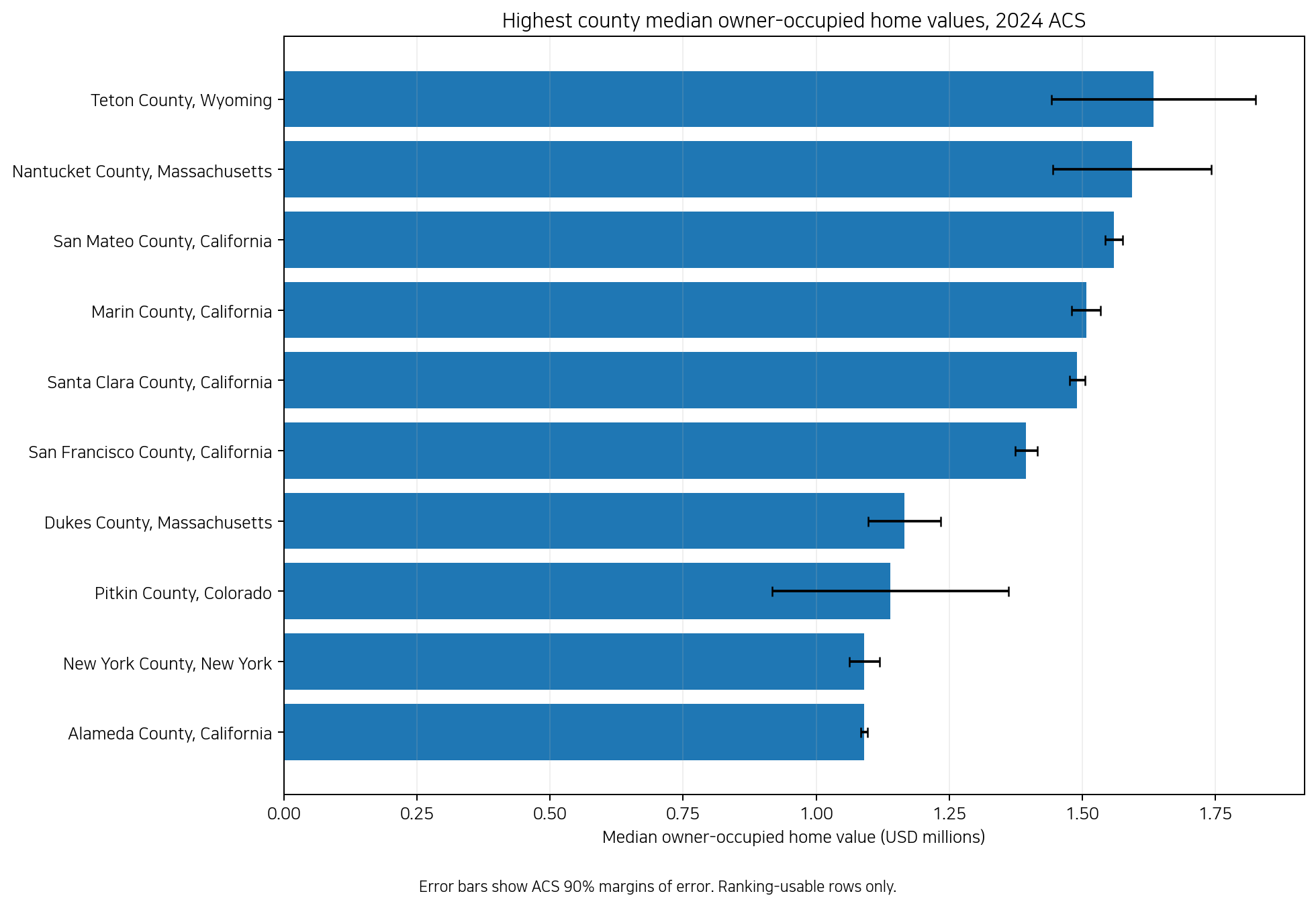
The margins of error are worth keeping beside the ranking. Teton County’s estimate has an MOE of about $191,937, while San Mateo County’s MOE is about $16,159. Both clearly sit in the high-value group, but the uncertainty is not equally large. A list that hides those intervals can make small rank differences look more precise than the survey supports.
Why the low end needs an uncertainty check
The lowest point estimates are not automatically the best candidates for a national “bottom ten” list. Stonewall County, Texas is estimated at $48,600, but its reliability status is CAUTION and ranking use is disabled. King County, Texas is similarly low at $52,100 and is also blocked from ranking because its uncertainty is large relative to the estimate.
| County | Median owner-occupied home value | 90% MOE |
|---|---|---|
| McDowell County, West Virginia | $50,000 | ±$4,822 |
| Oglala Lakota County, South Dakota | $52,900 | ±$7,539 |
| Cochran County, Texas | $53,200 | ±$14,031 |
| Todd County, South Dakota | $53,900 | ±$17,157 |
| Cottle County, Texas | $59,300 | ±$24,701 |
| Alexander County, Illinois | $59,800 | ±$7,126 |
| Apache County, Arizona | $63,700 | ±$3,664 |
| Hudspeth County, Texas | $64,000 | ±$12,904 |
Restricting the comparison to ranking-usable rows, McDowell County, West Virginia is lowest at $50,000. Oglala Lakota County, South Dakota is $52,900, Cochran County, Texas is $53,200, and Todd County, South Dakota is $53,900. The distance between the high and low ends is enormous, but the survey uncertainty is generally more important at the small-county end than a simple ordinal rank suggests.
Large differences can appear across a county line
The Census Bureau’s 2024 County Adjacency File makes it possible to compare counties that actually share a boundary rather than simply belong to the same state. Teton County, Wyoming is adjacent to Fremont, Lincoln, Park and Sublette counties in Wyoming, among others. Teton is estimated at $1,633,900, compared with $268,800 in Fremont, $372,600 in Lincoln, $400,500 in Park, and $376,200 in Sublette. The gap between Teton and adjacent Fremont is more than $1.36 million.
A different pattern appears among the high-value California counties. San Mateo County shares boundaries with San Francisco, Santa Clara, Santa Cruz and Alameda counties. San Mateo is $1,559,600, Santa Clara $1,490,600 and San Francisco $1,394,500, while Santa Cruz is $1,027,500 and Alameda $1,090,100. These neighboring counties form a high-value cluster, but the estimates still vary by hundreds of thousands of dollars inside that cluster.
At the low end, McDowell County, West Virginia is adjacent to Mercer and Wyoming counties in West Virginia and Tazewell County in Virginia. McDowell is $50,000, compared with $121,700 in Mercer, $82,900 in Wyoming County, and $118,300 in Tazewell. County borders therefore matter even in broadly low-value parts of the distribution.
A state summary helps show where high-value counties cluster
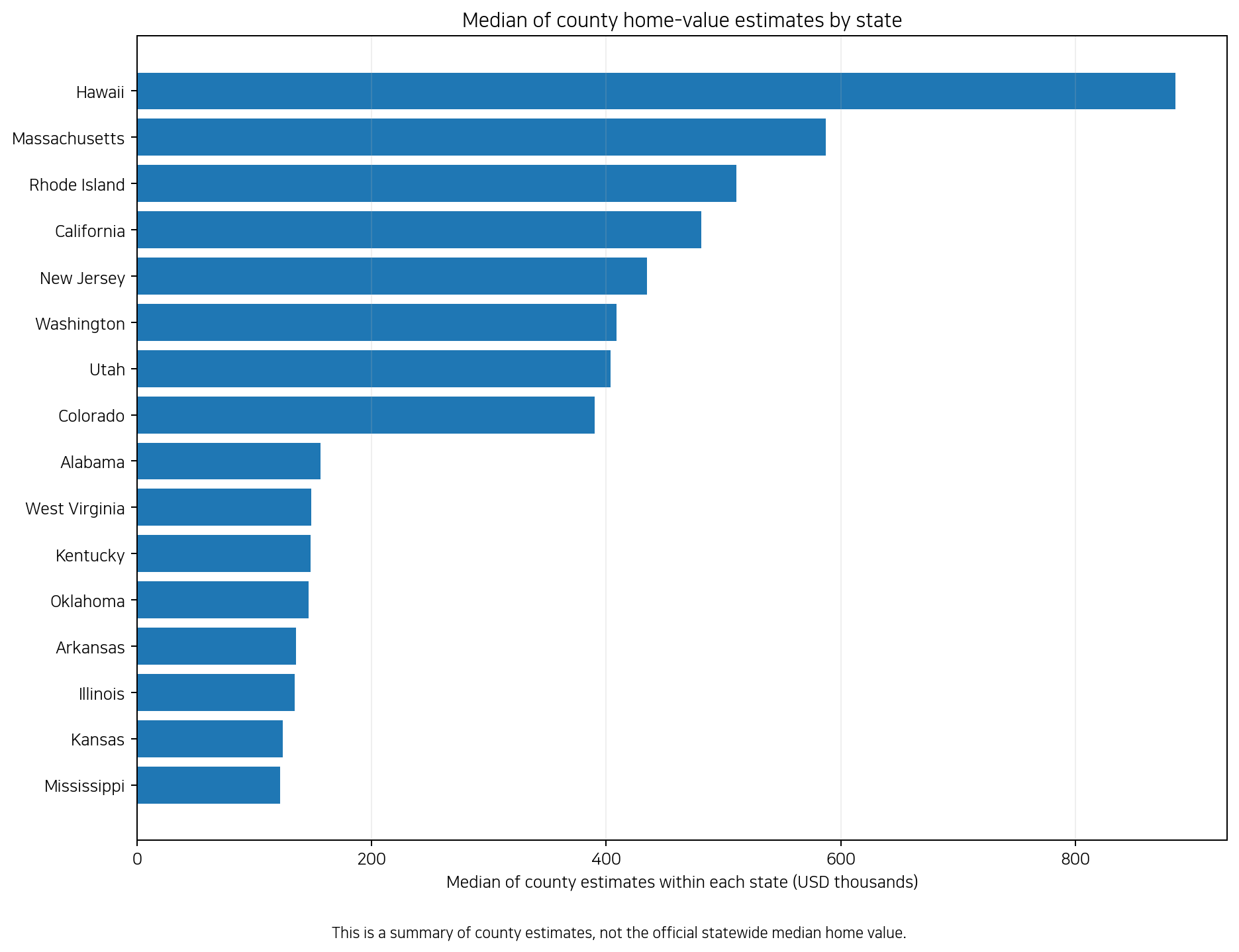
One way to summarize the map without replacing the county detail is to take the median of the county estimates within each state. This is an analysis derived from the county table, not the Census Bureau’s official statewide median home value. It answers a narrower question: what does the middle county estimate look like within each state?
By that measure, Hawaii’s county median is $885,350, Massachusetts is $587,550, Rhode Island is $510,800, and California is $481,100. At the lower end, Mississippi is $122,250, Kansas $124,200, Illinois $134,650, and Arkansas $135,700. California also has 29 of its 58 counties at or above $500,000, while Mississippi and Kansas have none at that threshold.
Coverage, missing estimates, and ranking reliability
The source geography has 3,144 rows. 3,139 are usable on the map and 3,123 are approved for ranking. The reliability field marks 3,123 rows as RELIABLE and 16 as CAUTION. Five county equivalents have no estimate: Kalawao County, Hawaii, plus Crockett, Edwards, Kenedy and Loving counties in Texas.
Missing estimates must be visually separated from low estimates. Treating a missing county as zero or placing it in the lowest color class would create a false geographic pattern. The same principle applies to rankings: a county can be valid for display but too uncertain for a precise ordinal comparison.
What the map does not say about affordability or future prices
A high median owner-occupied home value does not, by itself, establish high housing-cost burden. Affordability depends on household income and other costs, while renter pressure is measured with a different population and different variables. Likewise, a low median value is not proof of weak demand, economic distress, or easy affordability. Those claims require additional evidence.
The 2024 ACS 5-year estimate is also not a forecast. This map describes the cross-county pattern in one ACS product and does not show whether values are currently rising or falling. A trend article would need a matched earlier-year B25077 dataset and a carefully defined change calculation.
Source and method
Home-value estimates come from the U.S. Census Bureau 2024 ACS 5-year table B25077, variable B25077_001E. Values are in U.S. dollars and are keyed to 5-digit county GEOIDs. The published 90% margin of error is B25077_001M. The map includes only counties with usable estimates, and the ranking excludes rows that the supplied reliability review marked as unsuitable for ordinal comparison.
Neighbor comparisons use the U.S. Census Bureau’s 2024 County Adjacency File, which links each county GEOID to the county or county-equivalent GEOIDs it borders. That lets the article describe verified boundary-to-boundary contrasts instead of calling two places “neighbors” merely because they are in the same state.
- U.S. Census Bureau ACS 2024, Table B25077 – Median Value
- U.S. Census Bureau 2024 County Adjacency File
Frequently asked questions
Is this map showing actual home-sale prices?
No. It uses the ACS estimate for the median value of owner-occupied housing units. Recorded sale prices and monthly market indexes use different data and definitions.
Can every county estimate be used in a national ranking?
No. The dataset allows ranking for 3,123 rows. Counties with unusually large uncertainty and counties with no estimate should not be treated as equally precise rank observations.
Does a higher median home value mean housing is less affordable?
Not necessarily. Affordability requires income and housing-cost information in addition to home value, so this map should not be used as a stand-alone affordability ranking.
Related articles
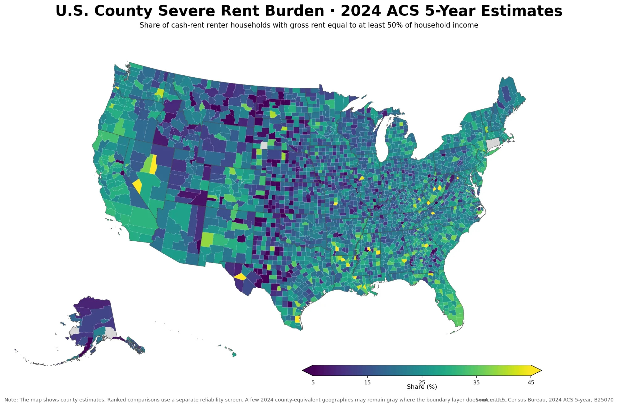
For a broader housing picture, compare the home-value level with county population growth, rent burden, and county boundary maps. Each article uses a different metric, so definitions and time periods should be checked before values are combined.
- U.S. County Population Growth vs Housing Costs Map, 2019–2024
- U.S. County Severe Rent Burden Map – Where Rent Takes Half of Income
- New York County Map Collection
Green Map creates custom-edited map images using open geographic data sources such as geoBoundaries, Natural Earth, OpenStreetMap, and government open data.
These maps are edited visual materials, not raw data files, and are provided for education, documents, presentations, and graphic reference.