Boone County, Kentucky, has two striking land-cover patterns: a large developed area on the eastern side and extensive wooded ground closer to the Ohio River. The supplied 2025 map classifies 39.47% of the county as forest, 31.35% as developed land, and 23.93% as agriculture. Those countywide shares become more meaningful when the colors are followed across the map rather than treated as a single average.
Four views are available here: overall land cover, forest and farmland, impervious surfaces, and mapped class differences from 1985 to 2025. Together they help compare the Florence-Hebron urban corridor with western river valleys and southern open land. The four original JPG maps can also be obtained in one ZIP archive for reference, presentations, or closer inspection.
Table of Contents
An eastern urban belt beside a wooded river county
Follow the outline of Boone County before interpreting individual colors. A curving western border follows the Ohio River, while the opposite side is edged by a comparatively straight boundary; dark green forest appears across substantial western and southwestern stretches. Farther east, connected red patches occupy a broad part of the map and become particularly dense toward the northern urban area.
Florence, Hebron, and Burlington provide familiar reference points for this landscape. The map itself shows categories, not municipal limits or labeled parcels; a developed cell can contain residential streets, paved commercial premises, or other human-modified ground. Nothing in the red color alone tells readers whether a particular parcel is zoned for housing, business, or industry.
A useful way to read this county is to compare the concentration of colors rather than only their total area. Forest leads the summary at 39.47%, yet it does not dominate every neighborhood. Developed cover reaches 31.35%, a substantial share concentrated much more heavily on the east. Agriculture forms a third major component, visible as scattered yellow fields and larger southern patches.
Geography offers context without proving a cause. Boone County’s comprehensive planning materials address land use, transportation, natural resources, and communities including Florence, Union, and Walton; they also discuss the Cincinnati/Northern Kentucky International Airport, commonly known as CVG. Those sources explain why urban and rural conditions both matter locally; this land-cover image should not be mistaken for the adopted plan’s zoning or future-land-use map.
Where hard surfaces become concentrated

Impervious surface is a measure of ground covered by materials that resist soaking up rainfall, including rooftops and pavement. In the third supplied image, white and very pale shades identify low impervious fractions, while orange and dark red indicate increasingly hard surfaces. Unlike the general cover map, this one separates more intensely paved cells from mixed cells that still contain vegetation.
The county summary gives an average impervious fraction of 11.12%. It also reports that 9.98% of the area falls in cells with at least 50% impervious cover. These figures describe different things. One is an average across the county. The other counts how much ground falls inside a high-intensity class. Neither percentage can be substituted for the developed-cover share of 31.35%.
Dark colors gather toward the northeastern and eastern portion of the county. That pattern is consistent with a broader built environment around the Florence-Hebron area and major transportation facilities. An individual red mark should not be labeled an airport runway, warehouse, or particular road without a matching reference map. The image offers a pattern of paved intensity, not a register of facilities.
Look west and the color distribution changes dramatically. Pale cells extend through much of the forested interior and toward the river-facing slopes. Fine orange traces remain visible within this lighter setting. Even so, the overall surface pattern differs from the crowded east. Comparing the impervious image with the forest-and-farmland view helps distinguish wooded ground from the places where roads and roofs are much more concentrated.
Between those broad regions is a mixed fringe. Pale and warm-colored pixels alternate rather than forming a perfectly sharp border. A pixel can contain both pavement and grass, so the displayed fraction changes gradually. In local drainage discussions, the map can identify areas worth a closer look, but it cannot estimate stormwater capacity or flood risk without topography, rainfall, and drainage-system evidence.
The general map: forests, development, fields, and the Ohio River

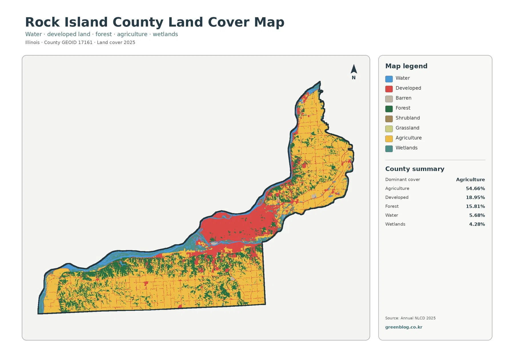
Begin with the main 2025 land-cover legend. Dark green represents forest, red represents developed cover, yellow represents agriculture, and blue represents open water. The county summary lists forest at 39.47%, developed cover at 31.35%, agriculture at 23.93%, water at 4.37%, and barren land at 0.48%. These are map classification shares, not population figures or measurements of legally designated land use.
Along the western edge, blue follows the bends of the Ohio River. Forested areas lie just inland, interrupted by small agricultural patches and narrow lighter strips. The boundary between vegetation types is irregular. River bends give way to inland slopes where the colors can change over short distances. A broad green block can contain narrow roads or clearings that are too small to appear as separate colors at this map scale.
Eastern Boone County looks markedly different. The developed class forms a relatively continuous area across portions of the northeast and east. Smaller green and yellow fragments remain within or beside it; this is not a statement that all the red-colored area is sealed under pavement; for that question, the fractional impervious map is the more appropriate image.
Agricultural yellow becomes especially visible farther south and southwest. Some fields appear in larger connected sections. Others interrupt the forest pattern as smaller openings. The resulting mosaic explains why a county with major urban facilities can still have an appreciable agricultural share. Field color does not specify a crop, farm ownership, or whether a property is actively cultivated on a particular date.
Small classes deserve care. Water is prominent along the county edge, while barren land is a much smaller component of the overall summary. The label ‘barren’ is a spectral or thematic cover category, not an announcement that a specific site is under construction. To discuss a particular clearing, readers would need recent aerial imagery and local information beyond this generalized map.
Forest and farmland across the western valleys

With the urban landscape pushed into a pale background, the forest-and-farmland map makes Boone County’s green and agricultural areas easier to distinguish. Forest remains dark green; yellow and light green tones separate cropland from pasture or hay, while water and wetlands have their own colors. The eastern developed area is intentionally less prominent in this view so that vegetation patterns can be examined more carefully.
A connected green network covers much of the western side. Near the Ohio River, the forest is interrupted by openings that vary in size and shape. Some openings resemble irregular fields rather than straight urban blocks; inland, narrow green corridors connect larger woodland sections in a pattern worth exploring on the original JPG. This image does not directly map elevation, so the viewer should not infer a precise slope from the color alone.
Agricultural cover accounts for 23.93% of the provided county summary. The category combines agricultural classes; it should not be read as a single crop type. Distinguishing cropland from pasture and hay allows a more useful question than simply asking whether a location is rural. Readers interested in crop production, stocking rates, or yields would need agricultural statistics, not the land-cover classification alone.
Southern Boone County has several notable transitions between fields and woods. Yellow patches meet green blocks repeatedly, and the pieces range from small clearings to broad areas. A forested polygon can sit directly beside land classed as agricultural, yet their adjacency does not establish ownership or management arrangements. County parcel records and property boundaries are separate information layers.
The map’s lesser categories also have a place. Its summary reports 0.21% grassland, 0.03% shrubland, and 0.17% wetlands, in addition to 4.37% water. Such small shares may look insignificant in a countywide graphic. At local scale, a wet area can still matter greatly for habitat or stream conditions. A thin riparian habitat may occupy only part of a mixed mapping cell.
Big Bone Lick State Historic Site offers a useful real-world example of why close-up context matters. Kentucky State Parks describes salt springs, wooded walking trails, and Big Bone Creek within the park. The county map cannot tell a viewer exactly where the park property line runs or identify each spring; pairing a site map with the broader vegetation image is a more responsible way to connect those features.
What changed in the classification between 1985 and 2025?

The change map compares two endpoints: 1985 and 2025. Light gray marks cells assigned the same mapped class, while red highlights cells categorized as changing to developed cover. Orange marks forest loss, yellow indicates agricultural-cover loss, and other colors identify wetland-related or remaining class differences. This legend must be read separately from the general 2025 map, where the same hues do not always carry the same message.
Across Boone County, the displayed total for mapped class differences is 24.50%. The summary breaks out 16.61% classified as a shift to developed cover, 1.99% forest loss, 1.07% agricultural loss, and 4.79% other differences. These categories describe the supplied comparison. They are not a record of permits, construction start dates, logging operations, or verified individual land transactions.
The strongest red concentration lies through the northeastern and eastern landscape. Its broad position overlaps the places where today’s developed cover and impervious colors are most conspicuous. That visual relationship helps readers see how the endpoint classifications differ in the urban belt. It does not prove that all identified changes happened simultaneously or arose from one economic project.
Elsewhere, smaller yellow and orange fragments interrupt extensive gray areas. Some occur near the boundary between wooded land and fields. At that boundary, classification can be sensitive to the surface visible in a particular year. Caution is particularly important when interpreting ‘forest loss’: the label describes a category transition, not necessarily a permanent disappearance of trees documented in the field.
A 40-year endpoint comparison cannot show every intermediate event. A location might have changed more than once, and the map would still summarize the difference between the two dates. Likewise, alternative classifications, sensor conditions, and product updates can influence results. Anyone pursuing a historical development timeline should examine dated imagery and the source documentation for each year of interest.
Use a precise caption if the percentages are reproduced in a report: ‘Share of Boone County with different mapped land-cover classes between the 1985 and 2025 endpoints.’ Saying that one-quarter of the county ‘was developed’ would be false. Even the 16.61% shift-to-developed class is a mapped change category. It is not a legal or engineering measure of new construction.
The river, Big Bone Creek, and the county's planning context
The Ohio River is a strong visual reference on the western side of the county. Water forms a blue border, while green woodland and yellow agricultural patches appear just inland. This pattern is useful for a watershed-oriented explanation of the landscape; yet the image does not show seasonal river stage, parcel-scale flood elevations, or the exact boundaries of protected riparian habitats.
At Big Bone Lick, local geography can be explored at a smaller scale than the county map allows. The Kentucky park description identifies trails, springs, and Big Bone Creek, together with a wooded setting; those features should not be located by guessing from a broad land-cover pixel. For on-site interpretation, the park’s own visitor materials provide the needed geographic detail.
Boone County’s adopted comprehensive planning framework considers natural resources, transportation, and future land-use choices. A classification map makes a useful background for those discussions because it reveals the contrast between eastern development and western tree cover. It remains an observation of surface conditions rather than a regulatory document. Consult the official plan for policy proposals and a current zoning map for permitted uses.
Choosing a JPG map for a particular question
A general overview works best with the land-cover image. Its full palette shows how forest, farmland, developed land, and river water occupy different parts of the county. In a classroom or presentation, begin with the eastern red belt and western green forest before introducing numbers. This location-first approach helps viewers avoid picturing 39.47% forest as evenly distributed everywhere. The percentage belongs to the county as a whole, not to every neighborhood.
For vegetation or rural-land discussions, the forest-and-farmland map offers more detail. Cropland and pasture or hay are separated, so the southern agricultural patches can be compared with western woodland and riverside cover. Keep the legend visible when cropping the graphic. Without it, a light green agricultural class might easily be mistaken for the darker forest class.
Impervious surfaces deserve their own slide when the topic is pavement, rooftops, or stormwater context. The 11.12% county average is meaningful only when contrasted with the much darker portions near eastern developed areas. It is not a substitute for storm-drain plans or runoff coefficients; where a particular project is involved, engineering surveys and site-specific information take precedence.
The change map suits a historical comparison, provided the time span is printed next to the illustration. Call out the 1985 and 2025 endpoints first. Then distinguish mapped shifts to developed cover from forest and agricultural losses. Avoid placing its red colors beside the general map without separate captions. A visually similar color does not always represent the same classification question.
These four images are supplied as original JPG maps in a single downloadable ZIP. Each includes its own map title, legend, and county summary. Use the original graphics for reference or print layout rather than capturing a small on-screen preview when fine text matters. The archive contains rendered map images, not an editable GIS project or certified boundary dataset.
Reading the maps without overclaiming
Annual NLCD classifies land from remotely sensed observations. Its underlying raster grid is commonly mapped at approximately 30 meters per cell. A cell may contain a road, grass, buildings, and trees. The displayed thematic class simplifies that mixture. A thin riverbank path or small commercial roof may therefore fail to appear as a distinct shape at county scale.
Another distinction is easy to miss: land cover describes the surface that the map classifies, while land use concerns how people manage or legally designate land. Yellow agricultural cover is not proof of farm ownership or a current crop. Red developed cover cannot establish zoning. For Boone County property decisions, consult official records, zoning maps, aerial photography, and appropriate field checks.
Water levels and vegetation appearance can change with seasons, particularly along the Ohio River and smaller creeks. The provided classification represents mapped conditions at its stated year, not a live view of every shoreline. Similarly, a change detected between 1985 and 2025 should not be presumed irreversible; a localized analysis benefits from several annual scenes, version notes, and ground verification.
USGS and MRLC publish the Annual NLCD classification descriptions and data-access documentation. The 2025 map here should be cited by its stated year, and a comparison with a different version should disclose the version difference. Historical releases and the newer Annual NLCD series are not automatically interchangeable; when precise measurements matter, obtain the underlying geospatial data and calculate areas using the documented methods.
Frequently Asked Questions
Is Boone County mostly forest or mostly urban?
Both descriptions capture only part of the story. Forest is the largest single mapped class at 39.47%, while developed cover accounts for another 31.35%. Most of the dense developed pattern lies toward the east and northeast, whereas broad western areas are wooded. Countywide percentages should always be read alongside the spatial pattern.
Why is impervious cover lower than developed cover?
The two measures are not equivalent. Developed land is a thematic class, while an impervious fraction estimates how much of a cell is occupied by hard surfaces such as pavement and rooftops. Boone County’s map reports 31.35% developed cover but an average impervious fraction of 11.12%. A developed location may still include lawns or trees.
Did 24.50% of Boone County become new construction after 1985?
No. The 24.50% figure covers all mapped class differences between the 1985 and 2025 endpoints. Shifts classified as developed account for 16.61%; forest, agricultural, and other differences are also recorded. The map does not verify construction permits, timing, or the cause of any individual transition.
What exactly comes in the four-map download?
The ZIP contains four original JPG graphics: the general land-cover map, forest-and-farmland map, impervious/developed-land map, and 1985–2025 land-cover change map. Each is a labeled image with a legend suitable for reference. The archive does not replace raw raster data, a surveyed boundary map, or a parcel-level planning record.
Sources and land-cover documentation
Figures quoted in this article come from the supplied map legends. The official resources below provide further documentation of classification methods, geographic boundaries, local planning, and natural features.
- Our Boone County — adopted 2045 comprehensive plan
- Kentucky State Parks — Big Bone Lick State Historic Site
- U.S. Geological Survey — Annual NLCD classification
- MRLC Consortium — Land Cover datasets
- National Park Service — Big Bone Lick site information
- U.S. Census Bureau — TIGER/Line boundary files
Map File Information
Download one ZIP archive containing the four original land-cover map JPG files.
- Included Files: Four original land-cover map JPG files
- File Type: ZIP archive containing four JPG files
- Intended Use: Map comparison, learning, and print reference
Related Maps
- Allen County Kentucky Land Cover Map
- Anderson County Kentucky Land Cover Map
- Cave Run Lake and the Wooded Hills: Bath County Kentucky Land Cover Map
Green Map creates custom-edited map images using open geographic data sources such as geoBoundaries, Natural Earth, OpenStreetMap, and government open data. These maps are edited visual materials, not raw data files, and are provided for education, documents, presentations, and graphic reference.