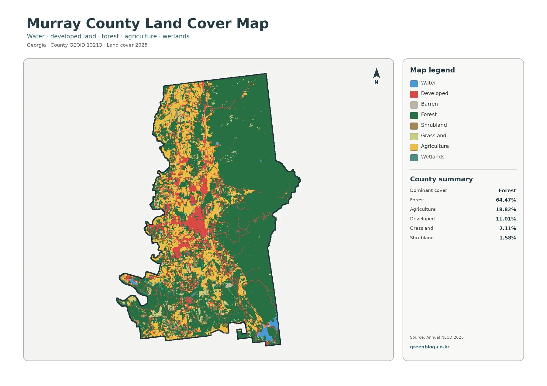
Kingman County Kansas Land Cover Maps place the county’s grassland and cultivated fields side by side. The 2025 overview assigns 49.28% of the area to grassland and 42.77% to agriculture. Dark, winding strips of vegetation interrupt the field grid, while the city of Kingman forms a compact developed cluster near the county’s middle.
Four views are available here: general land cover, forest and farmland, impervious and developed surfaces, and differences between the 1985 and 2025 classifications. The original four JPG maps come together in one ZIP archive. Their legends make it possible to compare a field, a stream corridor, and a town without treating those places as interchangeable.
Table of Contents
Start with the pattern, not the countywide percentage
Across Kingman County, pale green grassland and yellow agricultural cover form a patchwork. Individual field blocks have straighter edges than the vegetation bordering creeks. The distinction is easy to recognize in the northwest but remains visible through the southern half of the county. Neither land-cover class creates an uninterrupted region.
Grassland leads the map’s summary at 49.28%, narrowly ahead of agriculture at 42.77%. Together they account for most of the mapped surface. That balance matters more than choosing a single label for the county: some places are dominated by regular field blocks, whereas others have broader patches of open grass between farms.
Local geography helps explain what to inspect. Kingman County’s official website describes the area as predominantly prairie. It identifies the South Fork of the Ninnescah River across the north and the Chikaskia River in the south. Those named waterways provide a useful reference for following narrow ribbons of vegetation through the larger agricultural landscape.
The overall legend also gives developed cover as 5.13%, forest as 1.91%, and water as 0.52%. Small shares can still carry geographical weight. A green line beside a stream might be insignificant in a countywide area ranking but conspicuous when surrounded by square fields. The map invites both kinds of reading.

Follow the river corridors through the field grid
Near the northern part of the county, branching green and teal marks run across the agricultural grid. They are not a single broad forest. Wooded and wetland classes appear in narrow sections, often following curves rather than straight farm boundaries. Water and vegetation need to be read together because either class alone tells only part of the streamside story.
Southern parts of the map also contain winding strips and scattered short branches. Their form differs from the rectangular yellow blocks around them. A green strip may mark vegetation associated with a drainage, but the image alone cannot confirm whether a watercourse is perennial, seasonal, or part of a constructed channel.
The Chikaskia River passes through southern Kingman County according to the county’s geography page. Readers can use that verified place name when examining the stream-related patterns in the southern portion. Matching an individual pixel to a named tributary would require a separate hydrographic layer, however, not just a color key.
At the far northeastern corner, blue water stands out against a largely agricultural setting. Cheney Lake extends into that corner, as the county government notes. Its visible edge gives an accessible orientation point, but the colored boundary should not be mistaken for a legal shoreline or for a measurement of the lake at today’s water level.
The county also has Kingman State Fishing Lake and the Byron Walker wildlife area, both identified in official local descriptions. These places help readers understand why water and wildlife habitat matter locally. The land-cover image is not a recreational access map, so it should not be used to determine public entry points or fishing rules.
Cropland, prairie, and narrow belts of trees
An agricultural block is not simply an empty yellow rectangle. In the forest-and-farmland view, yellow cropland sits beside tan grass or shrub classes, while thin dark-green areas mark forest. The strongest visual contrast is between straight-edged fields and vegetation that follows drainage lines or irregular low-lying terrain.

The county summary lists agriculture at 42.77% and forest at 1.91%. These are mapped surface classes, not a count of farms or an inventory of every tree. Shelterbelts, tree rows, and small groves may be visible in photographs without reaching the threshold of a forest class in a generalized raster map.
Many field edges are relatively regular in the northern half. Farther south, brown and yellow surfaces remain mixed, and green lines break up the blocks where drainage vegetation appears. A reader tracing one field should pause where its boundary meets a wooded bend. That is often where the land-cover map becomes more informative than an undifferentiated satellite picture.
The distinction also matters for farming questions. A crop pixel does not identify wheat, sorghum, or any other specific crop. A grassland pixel does not prove that livestock graze it. Agricultural census records are needed to discuss farm operations, while the land-cover map answers which surface classes were detected in the imagery.
Kansas Department of Agriculture publishes a Kingman County profile using the 2022 Census of Agriculture. Its farm statistics describe a different measure and year from the 2025 cover classification. Keeping those sources separate avoids a misleading comparison between land-cover percentages and agricultural business activity.
Where impervious surfaces stand out
Roads, parking surfaces, and roofs can prevent rainwater from soaking into the ground. The impervious-surface map depicts that property in graduated classes rather than treating every settlement as fully paved. Light colors represent little mapped impervious cover. Stronger warm colors identify places with higher estimated proportions.

A concentrated warm-colored patch near the center and a little north of it aligns with the county seat, Kingman. An east–west corridor runs outward from that cluster. Smaller lines follow the rural road grid, while isolated warm spots appear at other developed locations across the county. This is a sparse network compared with the broad agricultural background.
Some minor red marks should be treated cautiously. Without street labels, a pixel does not establish the name of a small community, the owner of a structure, or whether a road has a particular pavement type. A current road map can provide those answers. Here the strength is the contrast between concentrated developed areas and the land surrounding them.
Three summary figures describe different things: mean imperviousness is 0.98%, the share mapped above 50% imperviousness is 0.24%, and developed cover is 5.13%. They are not interchangeable. The first concerns average surface coverage, the second identifies highly impervious locations, and the third refers to land-cover classification.
For example, a low-intensity developed cell can include vegetation beside homes or farm buildings. It may therefore belong to a developed class even without being mostly paved. Conversely, a narrow paved lane might blend with neighboring land within the mapping resolution. Avoid turning a single colored square into a parcel-level conclusion.
What the 1985–2025 comparison actually measures
The change view uses a very different palette. Much of Kingman County appears pale because the mapped class did not differ between the comparison years. Yellow patches denote a category involving agricultural loss; purple areas mark other class differences. Red represents places classified as developed in the later comparison, not all development that may have occurred in the county.

The supplied summary reports a 13.44% class difference. It lists 9.98% for agricultural loss, 0.69% for areas classified to developed, and 0.10% for forest loss. The remaining difference categories are described separately in the map legend. These percentages refer to classification differences, not directly to land transactions or employment.
Agricultural loss in the legend does not establish that the same share of farms closed. A pixel can shift between agricultural and grass cover because of real land-cover change, seasonal appearance, observation timing, or classification choices. The map provides a place to investigate, rather than an explanation by itself.
Many yellow marks are scattered across field-sized patches instead of forming a single outward-moving urban edge. That distribution argues against describing the whole 13.44% as urban expansion. Comparing the highlighted locations with time-specific imagery and county land records would be a more reliable way to investigate a particular site.
Read the comparison dates carefully. The current cover maps are labeled 2025, while the difference map compares 1985 and 2025. It is not a year-by-year animation. A cell that changed several times during the intervening years is reduced to a comparison between the two selected classifications.
Because the change map may include classification differences, not every colored patch should be described as confirmed physical conversion. The distinction is especially important where grassland and cultivated surfaces have similar seasonal appearances. More detailed field evidence is required before assigning a cause to a highlighted area.
A practical four-map reading route
Begin with a yellow field block in the 2025 cover map. Locate the same place in the forest-and-farmland view, where the adjacent grass and wooded strips are easier to separate. If a road passes nearby, check its footprint in the impervious layer. Finally, inspect the change view to see whether its class label differs from the 1985 comparison.
A second route starts at the city of Kingman. Impervious colors locate its compact built-up center. The general cover map then places that center against grassland and agricultural plots. In the change map, any colored cell nearby answers only whether the two mapped classes differ, not why a business or neighborhood developed.
For a third exercise, track a stream-related green ribbon rather than a town. Forest-and-farmland colors help reveal whether vegetation extends along the bends. The overall map adds water and wetlands. The developed-surface view can then show whether dense impervious cover occurs close to the same corridor, without claiming that a road caused any ecological condition.
These examples are useful in geography lessons because they require a reader to check more than one visual clue. Keep the legends and north arrows in view when comparing the graphics. A cropped image of the city alone would hide how small the developed component is relative to the rest of Kingman County.
For watershed discussion, a streamside vegetation pattern can guide the next research question. It cannot provide a water-quality result. Floodplains, erosion conditions, and regulated wetland boundaries need specialized datasets. Kansas has separate floodplain mapping resources that should be consulted for those purposes rather than inferred from green pixels.
Use the images as context, not as a survey
Each image is a representation of classified surface cover. Raster mapping places information into grid cells, and a single cell may contain more than one surface type. The output color summarizes a classification decision. A straight-looking line on the JPG does not necessarily match a property boundary, survey corner, or zoning district.
Annual NLCD products commonly use a 30-meter raster framework, but the JPG files here are cartographic images rather than editable source grids. Do not measure a land parcel from the JPG without verified scale and georeferenced source data. Map resolution and the level of detail visible on a screen are different concepts.
The same caution applies to woodland and wetland classes. Dark green does not demonstrate that a site meets a legal woodland definition, while teal does not establish jurisdictional wetland status. For any permit or conservation decision, seek the appropriate agency records and a site-specific assessment.
Aerial conditions may also change after the labeled imagery year. Road construction, seasonal water changes, planting, and vegetation growth can alter appearances without appearing on these graphics. The land-cover view is a dated reference, not a live monitoring service. Any high-stakes decision should use current official information.
The downloadable archive contains the original four JPG map graphics, each with a legend. Use them for side-by-side visual reference, education, or clearly labeled presentations. For analysis that requires pixel values, accurate area calculations, or intersections with property lines, obtain the underlying geospatial datasets and document the processing method.
Frequently Asked Questions
Is grassland or agriculture the largest land-cover class?
Grassland is the largest reported class at 49.28%, followed by agriculture at 42.77% in the supplied 2025 summary. The figures classify visible ground cover; they are not counts of ranches or harvested fields. Looking at both classes together is more informative than describing the county as exclusively prairie or cropland.
What explains the blue area at the northeastern edge?
The official Kingman County geography page says Cheney Lake reaches the county’s northeastern corner. The overview map also displays a blue water area there. The colored shoreline is a mapped surface class and should not be taken as a legal boundary or a measurement of today’s lake level.
Does the 9.98% agricultural-loss class mean 9.98% fewer farms?
No. It identifies cells assigned agriculture in one comparison and a different cover class in the other. The 1985–2025 comparison cannot establish a change in farm ownership, crop revenue, or farm numbers. Those questions require agricultural records and additional dated imagery.
Can the ZIP replace a parcel map or planning approval?
No. It contains four original JPG reference graphics, not surveyed parcel boundaries, a zoning determination, or authorization to develop land. Consult current county and state records before using these maps for legal, engineering, environmental, or real-estate decisions.
Sources and local context
- MRLC: Annual NLCD land-cover data
- USGS: Annual NLCD land-cover classes and definitions
- Kingman County government: geography, rivers and local lakes
- Kansas Department of Agriculture: Kingman County agricultural profile
- Kansas Department of Agriculture: Lower Arkansas floodplain mapping project
Map File Information
Download one ZIP archive containing the four original land-cover map JPG files.
- Included Files: Four original land-cover map JPG files
- File Type: ZIP archive containing four JPG files
- Intended Use: Map comparison, learning, and print reference
Related Maps
- Across the High Plains: Cheyenne County Kansas Land Cover Maps in Four Views
- Allen County Kansas Land Cover Maps | Fields, Iola and Four JPG Views
- Anderson County Kansas Land Cover Maps: Garnett, Wooded Creeks and Fields
Green Map creates custom-edited map images using open geographic data sources such as geoBoundaries, Natural Earth, OpenStreetMap, and government open data. These maps are edited visual materials, not raw data files, and are provided for education, documents, presentations, and graphic reference.